
The National Data Science Bowl, a data science competition where the goal was to classify images of plankton, has just ended. I participated with six other members of my research lab, the Reservoir lab of prof. Joni Dambre at Ghent University in Belgium. Our team finished 1st! In this post, we’ll explain our approach.

The ≋ Deep Sea ≋ team consisted of Aäron van den Oord, Ira Korshunova, Jeroen Burms, Jonas Degrave, Lionel Pigou, Pieter Buteneers and myself. We are all master students, PhD students and post-docs at Ghent University. We decided to participate together because we are all very interested in deep learning, and a collaborative effort to solve a practical problem is a great way to learn.
There were seven of us, so over the course of three months, we were able to try a plethora of different things, including a bunch of recently published techniques, and a couple of novelties. This blog post was written jointly by the team and will cover all the different ingredients that went into our solution in some detail.
Overview
This blog post is going to be pretty long! Here’s an overview of the different sections. If you want to skip ahead, just click the section title to go there.
- Introduction
- Pre-processing and data augmentation
- Network architecture
- Training
- Unsupervised and semi-supervised approaches
- Model averaging
- Miscellany
- Conclusion
Introduction
The problem
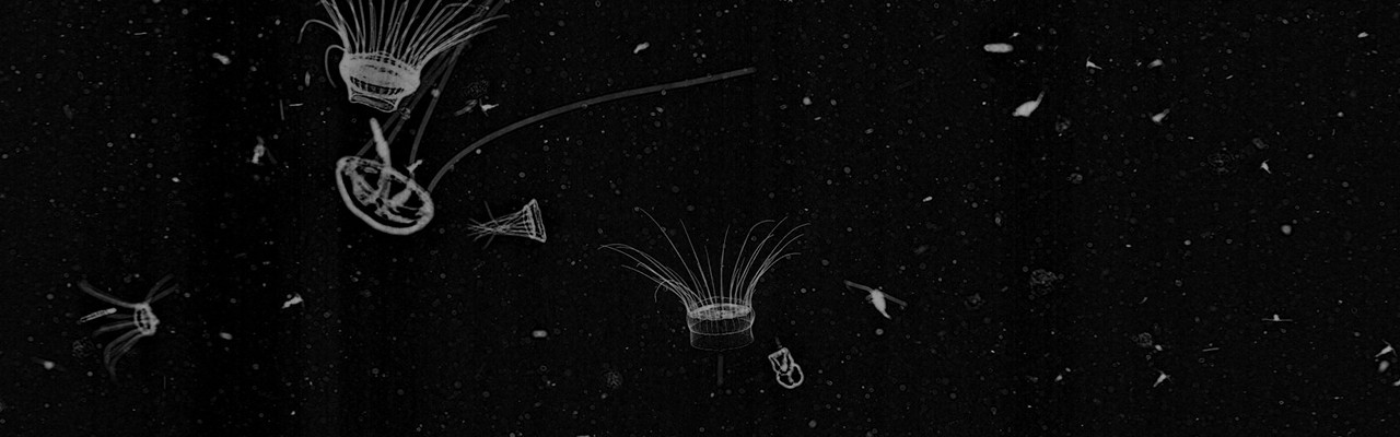
The goal of the competition was to classify grayscale images of plankton into one of 121 classes. They were created using an underwater camera that is towed through an area. The resulting images are then used by scientists to determine which species occur in this area, and how common they are. There are typically a lot of these images, and they need to be annotated before any conclusions can be drawn. Automating this process as much as possible should save a lot of time!
The images obtained using the camera were already processed by a segmentation algorithm to identify and isolate individual organisms, and then cropped accordingly. Interestingly, the size of an organism in the resulting images is proportional to its actual size, and does not depend on the distance to the lens of the camera. This means that size carries useful information for the task of identifying the species. In practice it also means that all the images in the dataset have different sizes.
Participants were expected to build a model that produces a probability distribution across the 121 classes for each image. These predicted distributions were scored using the log loss (which corresponds to the negative log likelihood or equivalently the cross-entropy loss).
This loss function has some interesting properties: for one, it is extremely sensitive to overconfident predictions. If your model predicts a probability of 1 for a certain class, and it happens to be wrong, the loss becomes infinite. It is also differentiable, which means that models trained with gradient-based methods (such as neural networks) can optimize it directly - it is unnecessary to use a surrogate loss function.
Interestingly, optimizing the log loss is not quite the same as optimizing classification accuracy. Although the two are obviously correlated, we paid special attention to this because it was often the case that significant improvements to the log loss would barely affect the classification accuracy of the models.
The solution: convnets!
Image classification problems are often approached using convolutional neural networks these days, and with good reason: they achieve record-breaking performance on some really difficult tasks.
A challenge with this competition was the size of the dataset: about 30000 examples for 121 classes. Several classes had fewer than 20 examples in total. Deep learning approaches are often said to require enormous amounts of data to work well, but recently this notion has been challenged, and our results in this competition also indicate that this is not necessarily true. Judicious use of techniques to prevent overfitting such as dropout, weight decay, data augmentation, pre-training, pseudo-labeling and parameter sharing, has enabled us to train very large models with up to 27 million parameters on this dataset.
Some of you may remember that I participated in another Kaggle competition last year: the Galaxy Challenge. The goal of that competition was to classify images of galaxies. It turns out that a lot of the things I learned during that competition were also applicable here. Most importantly, just like images of galaxies, images of plankton are (mostly) rotation invariant. I used this property for data augmentation, and incorporated it into the model architecture.
Software and hardware
We used Python, NumPy and Theano to implement our solution, in combination with the cuDNN library. We also used PyCUDA to implement a few custom kernels.
Our code is mostly based on the Lasagne library, which provides a bunch of layer classes and some utilities that make it easier to build neural nets in Theano. This is currently being developed by a group of researchers with different affiliations, including Aäron and myself. We hope to release the first version soon!
We also used scikit-image for pre-processing and augmentation, and ghalton for quasi-random number generation. During the competition, we kept track of all of our results in a Google Drive spreadsheet. Our code was hosted on a private GitHub repository, with everyone in charge of their own branch.
We trained our models on the NVIDIA GPUs that we have in the lab, which include GTX 980, GTX 680 and Tesla K40 cards.
Pre-processing and data augmentation
We performed very little pre-processing, other than rescaling the images in various ways and then performing global zero mean unit variance (ZMUV) normalization, to improve the stability of training and increase the convergence speed.
Rescaling the images was necessary because they vary in size a lot: the smallest ones are less than 40 by 40 pixels, whereas the largest ones are up to 400 by 400 pixels. We experimented with various (combinations of) rescaling strategies. For most networks, we simply rescaled the largest side of each image to a fixed length.
We also tried estimating the size of the creatures using image moments. Unfortunately, centering and rescaling the images based on image moments did not improve results, but they turned out to be useful as additional features for classification (see below).
Data augmentation
We augmented the data to artificially increase the size of the dataset. We used various affine transforms, and gradually increased the intensity of the augmentation as our models started to overfit more. We ended up with some pretty extreme augmentation parameters:
- rotation: random with angle between 0° and 360° (uniform)
- translation: random with shift between -10 and 10 pixels (uniform)
- rescaling: random with scale factor between 1/1.6 and 1.6 (log-uniform)
- flipping: yes or no (bernoulli)
- shearing: random with angle between -20° and 20° (uniform)
- stretching: random with stretch factor between 1/1.3 and 1.3 (log-uniform)
We augmented the data on-demand during training (realtime augmentation), which allowed us to combine the image rescaling and augmentation into a single affine transform. The augmentation was all done on the CPU while the GPU was training on the previous chunk of data.
We experimented with elastic distortions at some point, but this did not improve performance although it reduced overfitting slightly. We also tried sampling the augmentation transform parameters from gaussian instead of uniform distributions, but this did not improve results either.
Network architecture
Most of our convnet architectures were strongly inspired by OxfordNet: they consist of lots of convolutional layers with 3x3 filters. We used ‘same’ convolutions (i.e. the output feature maps are the same size as the input feature maps) and overlapping pooling with window size 3 and stride 2.
We started with a fairly shallow models by modern standards (~ 6 layers) and gradually added more layers when we noticed it improved performance (it usually did). Near the end of the competition, we were training models with up to 16 layers. The challenge, as always, was balancing improved performance with increased overfitting.
We experimented with strided convolutions with 7x7 filters in the first two layers for a while, inspired by the work of He et al., but we were unable to achieve the same performance with this in our networks.
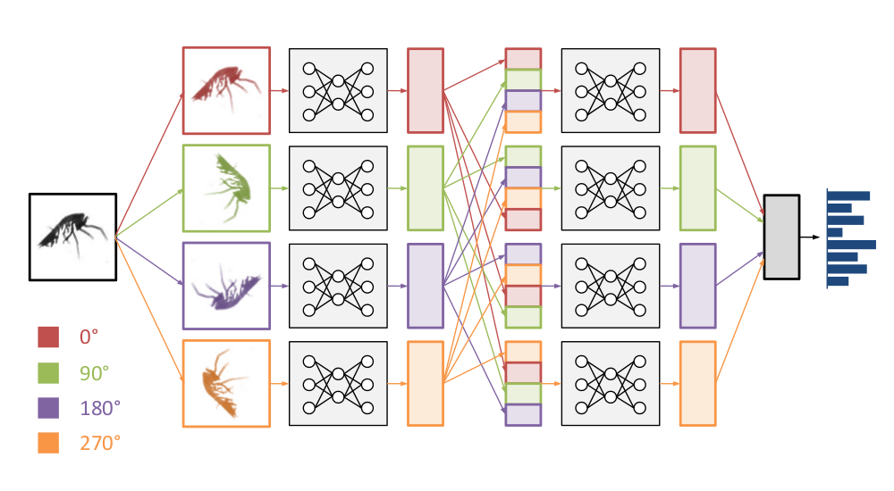
Cyclic pooling
When I participated in the Galaxy Challenge, one of the things I did differently from other competitors was to exploit the rotational symmetry of the images to share parameters in the network. I applied the same stack of convolutional layers to several rotated and flipped versions of the same input image, concatenated the resulting feature representations, and fed those into a stack of dense layers. This allowed the network to use the same feature extraction pipeline to “look at” the input from different angles.
Here, we took this a step further. Rather than concatenating the feature representations, we decided to pool across them to get rotation invariance. Here’s how it worked in practice: the images in a minibatch occur 4 times, in 4 different orientations. They are processed by the network in parallel, and at the top, the feature maps are pooled together. We decided to call this cyclic pooling, after cyclic groups.
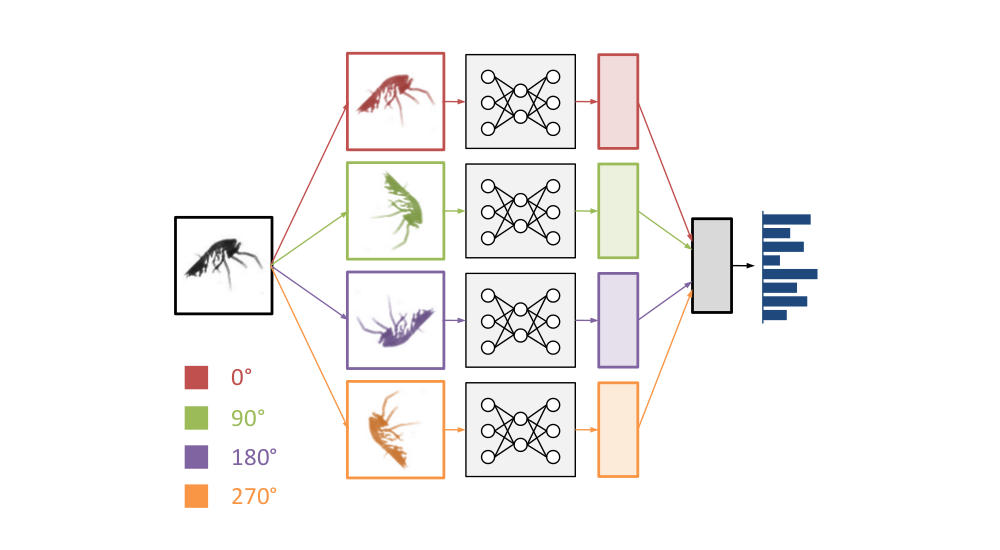
The nice thing about 4-way cyclic pooling is that it can be implemented very efficiently: the images are rotated by 0, 90, 180 and 270 degrees. All of these rotations can be achieved simply by transposing and flipping image axes. That means no interpolation is required.
Cyclic pooling also allowed us to reduce the batch size by a factor of 4: instead of having batches of 128 images, each batch now contained 32 images and was then turned into a batch with an effective size of 128 again inside the network, by stacking the original batch in 4 orientations. After the pooling step, the batch size was reduced to 32 again.
We tried several pooling functions over the course of the competition, as well as different positions in the network for the pooling operation (just before the output layer, between hidden layers, …). It turned out that root-mean-square pooling gave much better results than mean pooling or max pooling. We weren’t able to find a good explanation for this, but we suspect it may have something to do with rotational phase invariance.
One of our models pooled over 8 rotations, spaced apart 45 degrees. This required generating the input images at two angles (0 and 45 degrees). We also considered having the model do 8-way pooling by including flipped versions of each rotated image copy (dihedral pooling, after dihedral groups). Unfortunately this did not work better.
‘Rolling’ feature maps
Cyclic pooling modestly improved our results, but it can be taken a step further. A cyclic pooling convnet extracts features from input images in four different orientations. An alternative interpretation is that its filters are applied to the input images in four different orientations. That means we can combine the stacks of feature maps from the different orientations into one big stack, and then learn the next layer of features on this combined input. As a result, the network then appears to have 4 times more filters than it actually has!
This is cheap to do, since the feature maps are already being computed anyway. We just have to combine them together in the right order and orientation. We named the operation that combines feature maps from different orientations a roll.
Roll operations can be inserted after dense layers or after convolutional layers. In the latter case, care has to be taken to rotate the feature maps appropriately, so that they are all aligned.
We originally implemented the operations with a few lines of Theano code. This is a nice demonstration of Theano’s effectiveness for rapid prototyping of new ideas. Later on we spent some time implementing CUDA kernels for the roll operations and their gradients, because networks with many rolled layers were getting pretty slow to train. Using your own CUDA kernels with Theano turns out to be relatively easy in combination with PyCUDA. No additional C-code is required.
In most of the models we evaluated, we only inserted convolutional roll operations after the pooling layers, because this reduced the size of the feature maps that needed to be copied and stacked together.
Note that it is perfectly possible to build a cyclic pooling convnet without any roll operations, but it’s not possible to have roll operations in a network without cyclic pooling. The roll operation is only made possible because the cyclic pooling requires that each input image is processed in four different orientations to begin with.
Nonlinearities
We experimented with various variants of rectified linear units (ReLUs), as well as maxout units (only in the dense layers). We also tried out smooth non-linearities and the ‘parameterized ReLUs’ that were recently introduced by He et al., but found networks with these units to be very prone to overfitting.
However, we had great success with (very) leaky ReLUs. Instead of taking the maximum of the input and zero, y = max(x, 0), leaky ReLUs take the maximum of the input and a scaled version of the input, y = max(x, a*x). Here, a is a tunable scale parameter. Setting it to zero yields regular ReLUs, and making it trainable yields parameterized ReLUs.
For fairly deep networks (10+ layers), we found that varying this parameter between 0 and 1/2 did not really affect the predictive performance. However, larger values in this range significantly reduced the level of overfitting. This in turn allowed us to scale up our models further. We eventually settled on a = 1/3.
Spatial pooling
We started out using networks with 2 or 3 spatial pooling layers, and we initially had some trouble getting networks with more pooling stages to work well. Most of our final models have 4 pooling stages though.
We started out with the traditional approach of 2x2 max-pooling, but eventually switched to 3x3 max-pooling with stride 2 (which we’ll refer to as 3x3s2), mainly because it allowed us to use a larger input size while keeping the same feature map size at the topmost convolutional layer, and without increasing the computational cost significantly.
As an example, a network with 80x80 input and 4 2x2 pooling stages will have feature maps of size 5x5 at the topmost convolutional layer. If we use 3x3s2 pooling instead, we can feed 95x95 input and get feature maps with the same 5x5 shape. This improved performance and only slowed down training slightly.
Multiscale architectures
As mentioned before, the images vary widely in size, so we usually rescaled them using the largest dimension of the image as a size estimate. This is clearly suboptimal, because some species of plankton are larger than others. Size carries valuable information.
To allow the network to learn this, we experimented with combinations of different rescaling strategies within the same network, by combining multiple networks with different rescaled inputs together into ‘multiscale’ networks.
What worked best was to combine a network with inputs rescaled based on image size, and a smaller network with inputs rescaled by a fixed factor. Of course this slowed down training quite a bit, but it allowed us to squeeze out a bit more performance.
Additional image features
We experimented with training small neural nets on extracted image features to ‘correct’ the predictions of our convnets. We referred to this as ‘late fusing’ because the feature network and the convnet were joined only at the output layer (before the softmax). We also tried joining them at earlier layers, but consistently found this to work worse, because of overfitting.
We thought this could be useful, because the features can be extracted from the raw (i.e. non-rescaled) images, so this procedure could provide additional information that is missed by the convnets. Here are some examples of types of features we evaluated (the ones we ended up using are in bold):
- Image size in pixels
- Size and shape estimates based on image moments
- Hu moments
- Zernike moments
- Parameter Free Threshold Adjacency Statistics
- Linear Binary Patterns
- Haralick texture features
- Features from the competition tutorial
- Combinations of the above
The image size, the features based on image moments and the Haralick texture features were the ones that stood out the most in terms of performance. The features were fed to a neural net with two dense layers of 80 units. The final layer of the model was fused with previously generated predictions of our best convnet-based models. Using this approach, we didn’t have to retrain the convnets nor did we have to regenerate predictions (which saved us a lot of time).
To deal with variance due to the random weight initialization, we trained each feature network 10 times and blended the copies with uniform weights. This resulted in a consistent validation loss decrease of 0.01 (or 1.81%) on average, which was quite significant near the end of the competition.
Interestingly, late fusion with image size and features based on image moments seems to help just as much for multiscale models as for regular convnets. This is a bit counterintuitive: we expected both approaches to help because they could extract information about the size of the creatures, so the obtained performance improvements would overlap. The fact they were fully orthogonal was a nice surprise.
Example convnet architecture
Here’s an example of an architecture that works well. It has 13 layers with parameters (10 convolutional, 3 fully connected) and 4 spatial pooling layers. The input shape is (32, 1, 95, 95), in bc01 order (batch size, number of channels, height, width). The output shape is (32, 121). For a given input, the network outputs 121 probabilities that sum to 1, one for each class.
| Layer type | Size | Output shape |
|---|---|---|
| cyclic slice | (128, 1, 95, 95) | |
| convolution | 32 3x3 filters | (128, 32, 95, 95) |
| convolution | 16 3x3 filters | (128, 16, 95, 95) |
| max pooling | 3x3, stride 2 | (128, 16, 47, 47) |
| cyclic roll | (128, 64, 47, 47) | |
| convolution | 64 3x3 filters | (128, 64, 47, 47) |
| convolution | 32 3x3 filters | (128, 32, 47, 47) |
| max pooling | 3x3, stride 2 | (128, 32, 23, 23) |
| cyclic roll | (128, 128, 23, 23) | |
| convolution | 128 3x3 filters | (128, 128, 23, 23) |
| convolution | 128 3x3 filters | (128, 128, 23, 23) |
| convolution | 64 3x3 filters | (128, 64, 23, 23) |
| max pooling | 3x3, stride 2 | (128, 64, 11, 11) |
| cyclic roll | (128, 256, 11, 11) | |
| convolution | 256 3x3 filters | (128, 256, 11, 11) |
| convolution | 256 3x3 filters | (128, 256, 11, 11) |
| convolution | 128 3x3 filters | (128, 128, 11, 11) |
| max pooling | 3x3, stride 2 | (128, 128, 5, 5) |
| cyclic roll | (128, 512, 5, 5) | |
| fully connected | 512 2-piece maxout units | (128, 512) |
| cyclic pooling (rms) | (32, 512) | |
| fully connected | 512 2-piece maxout units | (32, 512) |
| fully connected | 121-way softmax | (32, 121) |
Note how the ‘cyclic slice’ layer increases the batch size fourfold. The ‘cyclic pooling’ layer reduces it back to 32 again near the end. The ‘cyclic roll’ layers increase the number of feature maps fourfold.
Training
Validation
We split off 10% of the labeled data as a validation set using stratified sampling. Due to the small size of this set, our validation estimates were relatively noisy and we periodically validated some models on the leaderboard as well.
Training algorithm
We trained all of our models with stochastic gradient descent (SGD) with Nesterov momentum. We set the momentum parameter to 0.9 and did not tune it further. Most models took between 24 and 48 hours to train to convergence.
We trained most of the models with about 215000 gradient steps and eventually settled on a discrete learning rate schedule with two 10-fold decreases (following Krizhevsky et al.), after about 180000 and 205000 gradient steps respectively. For most models we used an initial learning rate of 0.003.
We briefly experimented with the Adam update rule proposed by Kingma and Ba, as an alternative to Nesterov momentum. We used the version of the algorithm described in the first version of the paper, without the lambda parameter. Although this seemed to speed up convergence by a factor of almost 2x, the results were always slightly worse than those achieved with Nesterov momentum, so we eventually abandoned this idea.
Initialization
We used a variant of the orthogonal initialization strategy proposed by Saxe et al. everywhere. This allowed us to add as many layers as we wanted without running into any convergence problems.
Regularization
For most models, we used dropout in the fully connected layers of the network, with a dropout probability of 0.5. We experimented with dropout in the convolutional layers as well for some models.
We also tried Gaussian dropout (using multiplicative Gaussian noise instead of multiplicative Bernoulli noise) and found this to work about as well as traditional dropout.
We discovered near the end of the competition that it was useful to have a small amount of weight decay to stabilize training of larger models (so not just for its regularizing effect). Models with large fully connected layers and without weight decay would often diverge unless the learning rate was decreased considerably, which slowed things down too much.
Unsupervised and semi-supervised approaches
Unsupervised pre-training
Since the test set was much larger than the training set, we experimented with using unsupervised pre-training on the test set to initialize the networks. We only pre-trained the convolutional layers, using convolutional auto-encoders (CAE, Masci. et al.). This approach consists of building a stack of layers implementing the reverse operations (i.e. deconvolution and unpooling) of the layers that are to be pre-trained. These can then be used to try and reconstruct the input of those layers.
In line with the literature, we found that pre-training a network serves as an excellent regularizer (much higher train error, slightly better validation score), but the validation results with test-time augmentation (see below) were consistently slightly worse for some reason.
Pre-training might allow us to scale our models up further, but because they already took a long time to train, and because the pre-training itself was time-consuming as well, we did not end up doing this for any of our final models.
To learn useful features with unsupervised pre-training, we relied on the max-pooling and unpooling layers to serve as a sparsification of the features. We did not try a denoising autoencoder approach for two reasons: first of all, according to the results described by Masci et al., the max- and unpooling approach produces way better filters than the denoising approach, and the further improvement of combining these approaches is negligible. Secondly, due to how the networks were implemented, it would slow things down a lot.
We tried different setups for this pre-training stage:
- greedy layerwise training vs. training the full deconvolutional stack jointly: we obtained the best results when pre-training the full stack jointly. Sometimes it was necessary to initialize this stack using the greedy approach to get it to work.
- using tied weights vs. using untied weights: Having the weights in the deconvolutional layers be the transpose of those in the corresponding convolutional layers made the (full) autoencoder easier and much faster to train. Because of this, we never got the CAE with untied weights to reconstruct the data as well as the CAE with tied weights, despite having more trainable parameters.
We also tried different approaches for the supervised finetuning stage. We observed that without some modifications to our supervised training setup, there was no difference in performance between a pre-trained network and a randomly initialized one. Possibly, by the time the randomly initialized dense layers are in a suitable parameter range, the network has already forgotten a substantial amount of the information it acquired during the pre-training phase.
We found two ways to overcome this:
-
keeping the pre-trained layers fixed for a while: before training the full networks, we only train the (randomly initialized) dense layers. This is quite fast since we only need to backpropagate through the top few layers. The idea is that we put the network more firmly in the basin of attraction the pre-training led us to.
-
Halving the learning rate in the convolutional layers: By having the dense layers adapt faster to the (pre-trained) convolutional layers, the network is less likely to make large changes to the pre-trained parameters before the dense layers are in a good parameter range.
Both approaches produced similar results.
Pseudo-labeling
Another way we exploited the information in the test set was by a combination of pseudo-labeling and knowledge distillation (Hinton et al.). The initial results from models trained with pseudo-labeling were significantly better than we anticipated, so we ended up investigating this approach quite thoroughly.
Pseudo-labeling entails adding test data to the training set to create a much larger dataset. The labels of the test datapoints (so called pseudo-labels) are based on predictions from a previously trained model or an ensemble of models. This mostly had a regularizing effect, which allowed us to train bigger networks.
We experimented both with hard targets (one-hot coded) and soft targets (predicted probabilities), but quickly settled on soft targets as these gave much better results.
Another important detail is the balance between original data and pseudo-labeled data in the resulting dataset. In most of our experiments 33% of the minibatch was sampled from the pseudolabeled dataset and 67% from the real training set.
It is also possible to use more pseudo-labeled data points (e.g. 67%). In this case the model is regularized a lot more, but the results will be more similar to the pseudolabels. As mentioned before, this allowed us to train bigger networks, but in fact this is necessary to make pseudo-labeling work well. When using 67% of the pseudo-labeled dataset we even had to reduce or disable dropout, or the models would underfit.
Our pseudo-labeling approach differs from knowledge distillation in the sense that we use the test set instead of the training set to transfer knowledge between models. Another notable difference is that knowledge distillation is mainly intended for training smaller and faster networks that work nearly as well as bigger models, whereas we used it to train bigger models that perform better than the original model(s).
We think pseudo-labeling helped to improve our results because of the large test set and the combination of data-augmentation and test-time augmentation (see below). When pseudo-labeled test data is added to the training set, the network is optimized (or constrained) to generate predictions similar to the pseudo-labels for all possible variations and transformations of the data resulting from augmentation. This makes the network more invariant to these transformations, and forces the network to make more meaningful predictions.
We saw the biggest gains in the beginning (up to 0.015 improvement on the leaderboard), but even in the end we were able to improve on very large ensembles of (bagged) models (between 0.003 - 0.009).
Model averaging
We combined several forms of model averaging in our final submissions.
Test-time augmentation
For each individual model, we computed predictions across various augmented versions of the input images and averaged them. This improved performance by quite a large margin. When we started doing this, our leaderboard score dropped from 0.7875 to 0.7081. We used the acronym TTA to refer to this operation.
Initially, we used a manually created set of affine transformations which were applied to each image to augment it. This worked better than using a set of transformations with randomly sampled parameters. After a while, we looked for better ways to tile the augmentation parameter space, and settled on a quasi-random set of 70 transformations, using slightly more modest augmentation parameter ranges than those used for training.
Computing model predictions for the test set using TTA could take up to 12 hours, depending on the model.
Finding the optimal transformation instead of averaging
Since the TTA procedure improved the score considerably, we considered the possibility of optimizing the augmentation parameters at prediction time. This is possible because affine transformations are differentiable with respect to their parameters.
In order to do so, we implemented affine transformations as layers in a network, so that we could backpropagate through them. After the transformation is applied to an image, a pixel can land in between two positions of the pixel grid, which makes interpolation necessary. This makes finding these derivatives quite complex.
We tried various approaches to find the optimal augmentation, including the following:
- Optimizing the transformation parameters to maximize (or minimize) the confidence of the predictions.
- Training a convnet to predict the optimal transformation parameters for another convnet to use.
Unfortunately we were not able to improve our results with any of these approaches. This may be because selecting an optimal input augmentation as opposed to averaging across augmentations removes the regularizing effect of the averaging operation. As a consequence we did not use this technique in our final submissions, but we plan to explore this idea further.
Combining different models
In total we trained over 300 models, so we had to select how many and which models to use in the final blend. For this, we used cross-validation on our validation set. On each fold, we optimized the weights of all models to minimize the loss of the ensemble on the training part.
We regularly created new ensembles from a different number of top-weighted models, which we further evaluated on the testing part. In the end, this could give an approximate idea of suitable models for ensembling.
Once the models were selected, they were blended uniformly or with weights optimized on the validation set. Both approaches gave comparable results.
The models selected by this process were not necessarily the ones with the lowest TTA score. Some models with relatively poor scores were selected because they make very different predictions than our other models. A few models had poor scores due to overfitting, but were selected nevertheless because the averaging reduces the effect of overfitting.
Bagging
To improve the score of the ensemble further, we replaced some of the models by an average of 5 models (including the original one), where each model was trained on a different subset of the data.
Miscellany
Here are a few other things we tried, with varying levels of success:
- untied biases: having separate biases for each spatial location in the convolutional layer seemed to improve results very slightly.
- winner take all nonlinearity (WTA, also known as channel-out) in the fully connected layers instead of ReLUs / maxout.
- smooth nonlinearities: to increase the amount of variance in our blends we tried replacing the leaky rectified linear units with a smoothed version. Unfortunately this worsened our public leaderboard score.
- specialist models: we tried training special models for highly confusable classes of chaetognaths, some protists, etc. using the knowledge distillation approach described by Hinton et al.. We also tried a self-informed neural network structure learning (Warde-Farley et al.), but in both cases the improvements were negligible.
- batch normalization: unfortunately we were unable to reproduce the spectacular improvements in convergence speed described by Ioffe and Szegedy for our models.
- Using FaMe regularization as described by Rudy et al. instead of dropout increased overfitting a lot. The regularizing effect seemed to be considerably weaker.
- Semi-supervised learning with soft and hard bootstrapping as described by Reed et al. did not improve performance or reduce overfitting.
Here’s a non-exhaustive list of things that we found to reduce overfitting (including the obvious ones):
- dropout (various forms)
- aggressive data augmentation
- suitable model architectures (depth and width of the layers influence overfitting in complicated ways)
- weight decay
- unsupervised pre-training
- cyclic pooling (especially with root-mean-square pooling)
- leaky ReLUs
- pseudo-labeling
We also monitored the classification accuracy of our models during the competition. Our best models achieved an accuracy of over 82% on the validation set, and a top-5 accuracy of over 98%. This makes it possible to use the model as a tool for speeding up manual annotation.
Conclusion
We had a lot of fun working on this problem together and learned a lot! If this problem interests you, be sure to check out the competition forum. Many of the participants will be posting overviews of their approaches in the coming days.
Congratulations to the other winners, and our thanks to the competition organizers and sponsors. We would also like to thank our supervisor Joni Dambre for letting us work on this problem together.
We will clean up our code and put it on GitHub soon. If you have any questions or feedback about this post, feel free to leave a comment.
One of our team, Ira Korshunova, is currently looking for a good research lab to start her PhD next semester. She can be contacted at irene.korshunova@gmail.com.
UPDATE (March 25th): the code is now available on GitHub: https://github.com/benanne/kaggle-ndsb
