Guidance is a powerful method that can be used to enhance diffusion model sampling. As I’ve discussed in an earlier blog post, it’s almost like a cheat code: it can improve sample quality so much that it’s as if the model had ten times the number of parameters – an order of magnitude improvement, basically for free! This follow-up post provides a geometric interpretation and visualisation of the diffusion sampling procedure, which I’ve found particularly useful to explain how guidance works.
A word of warning about high-dimensional spaces
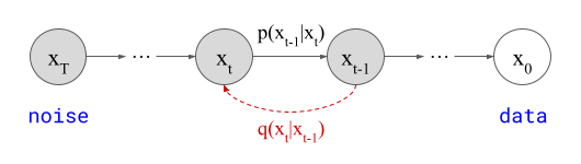
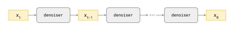
Sampling algorithms for diffusion models typically start by initialising a canvas with random noise, and then repeatedly updating this canvas based on model predictions, until a sample from the model distribution eventually emerges.
We will represent this canvas by a vector \(\mathbf{x}_t\), where \(t\) represents the current time step in the sampling procedure. By convention, the diffusion process which gradually corrupts inputs into random noise moves forward in time from \(t=0\) to \(t=T\), so the sampling procedure goes backward in time, from \(t=T\) to \(t=0\). Therefore \(\mathbf{x}_T\) corresponds to random noise, and \(\mathbf{x}_0\) corresponds to a sample from the data distribution.
\(\mathbf{x}_t\) is a high-dimensional vector: for example, if a diffusion model produces images of size 64x64, there are 12,288 different scalar intensity values (3 colour channels per pixel). The sampling procedure then traces a path through a 12,288-dimensional Euclidean space.
It’s pretty difficult for the human brain to comprehend what that actually looks like in practice. Because our intuition is firmly rooted in our 3D surroundings, it actually tends to fail us in surprising ways in high-dimensional spaces. A while back, I wrote a blog post about some of the implications for high-dimensional probability distributions in particular. This note about why high-dimensional spheres are “spikey” is also worth a read, if you quickly want to get a feel for how weird things can get. A more thorough treatment of high-dimensional geometry can be found in chapter 2 of ‘Foundations of Data Science’1 by Blum, Hopcroft and Kannan, which is available to download in PDF format.
Nevertheless, in this blog post, I will use diagrams that represent \(\mathbf{x}_t\) in two dimensions, because unfortunately that’s all the spatial dimensions available on your screen. This is dangerous: following our intuition in 2D might lead us to the wrong conclusions. But I’m going to do it anyway, because in spite of this, I’ve found these diagrams quite helpful to explain how manipulations such as guidance affect diffusion sampling in practice.
Here’s some advice from Geoff Hinton on dealing with high-dimensional spaces that may or may not help:
I'm laughing so hard at this slide a friend sent me from one of Geoff Hinton's courses;
— Robbie Barrat (@videodrome) June 10, 2018
"To deal with hyper-planes in a 14-dimensional space, visualize a 3-D space and say 'fourteen' to yourself very loudly. Everyone does it." pic.twitter.com/nTakZArbsD
… anyway, you’ve been warned!
Visualising diffusion sampling
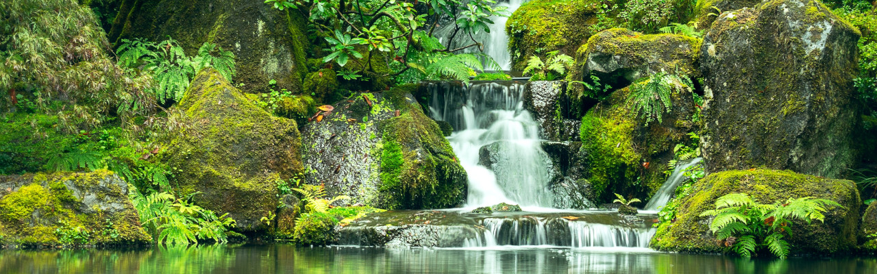
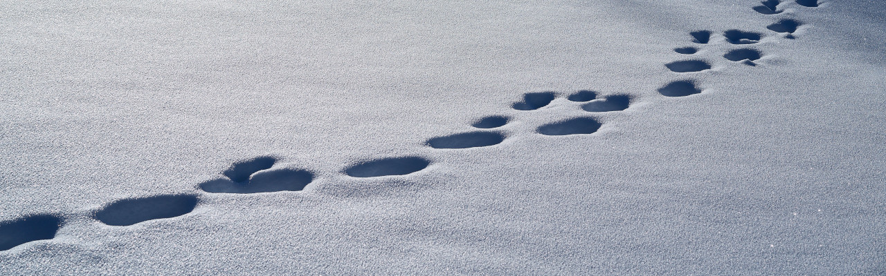
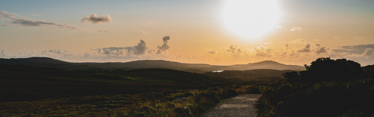
To start off, let’s visualise what a step of diffusion sampling typically looks like. I will use a real photograph to which I’ve added varying amounts of noise to stand in for intermediate samples in the diffusion sampling process:
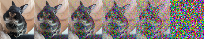
During diffusion model training, examples of noisy images are produced by taking examples of clean images from the data distribution, and adding varying amounts of noise to them. This is what I’ve done above. During sampling, we start from a canvas that is pure noise, and then the model gradually removes random noise and replaces it with meaningful structure in accordance with the data distribution. Note that I will be using this set of images to represent intermediate samples from a model, even though that’s not how they were constructed. If the model is good enough, you shouldn’t be able to tell the difference anyway!
In the diagram below, we have an intermediate noisy sample \(\mathbf{x}_t\), somewhere in the middle of the sampling process, as well as the final output of that process \(\mathbf{x}_0\), which is noise-free:

Imagine the two spatial dimensions of your screen representing just two of many thousands of pixel colour intensities (red, green or blue). Different spatial positions in the diagram correspond to different images. A single step in the sampling procedure is taken by using the model to predict where the final sample will end up. We’ll call this prediction \(\hat{\mathbf{x}}_0\):
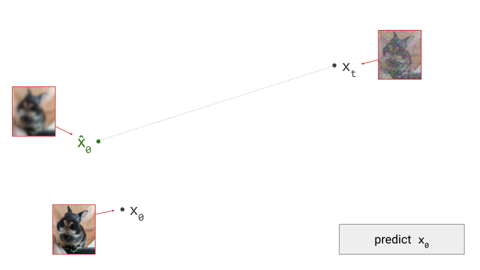
Note how this prediction is roughly in the direction of \(\mathbf{x}_0\), but we’re not able to predict \(\mathbf{x}_0\) exactly from the current point in the sampling process, \(\mathbf{x}_t\), because the noise obscures a lot of information (especially fine-grained details), which we aren’t able to fill in all in one go. Indeed, if we were, there would be no point to this iterative sampling procedure: we could just go directly from pure noise \(\mathbf{x}_T\) to a clean image \(\mathbf{x}_0\) in one step. (As an aside, this is more or less what Consistency Models2 try to achieve.)
Diffusion models estimate the expectation of \(\mathbf{x}_0\), given the current noisy input \(\mathbf{x}_t\): \(\hat{\mathbf{x}}_0 = \mathbb{E}[\mathbf{x}_0 \mid \mathbf{x}_t]\). At the highest noise levels, this expectation basically corresponds to the mean of the entire dataset, because very noisy inputs are not very informative. As a result, the prediction \(\hat{\mathbf{x}}_0\) will look like a very blurry image when visualised. At lower noise levels, this prediction will become sharper and sharper, and it will eventually resemble a sample from the data distribution. In a previous blog post, I go into a little bit more detail about why diffusion models end up estimating expectations.
In practice, diffusion models are often parameterised to predict noise, rather than clean input, which I also discussed in the same blog post. Some models also predict time-dependent linear combinations of the two. Long story short, all of these parameterisations are equivalent once the model has been trained, because a prediction of one of these quantities can be turned into a prediction of another through a linear combination of the prediction itself and the noisy input \(\mathbf{x}_t\). That’s why we can always get a prediction \(\hat{\mathbf{x}}_0\) out of any diffusion model, regardless of how it was parameterised or trained: for example, if the model predicts the noise, simply take the noisy input and subtract the predicted noise.
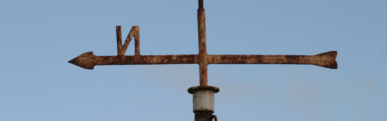
Diffusion model predictions also correspond to an estimate of the so-called score function, \(\nabla_{\mathbf{x}_t} \log p(\mathbf{x}_t)\). This can be interpreted as the direction in input space along which the log-likelihood of the input increases maximally. In other words, it’s the answer to the question: “how should I change the input to make it more likely?” Diffusion sampling now proceeds by taking a small step in the direction of this prediction:
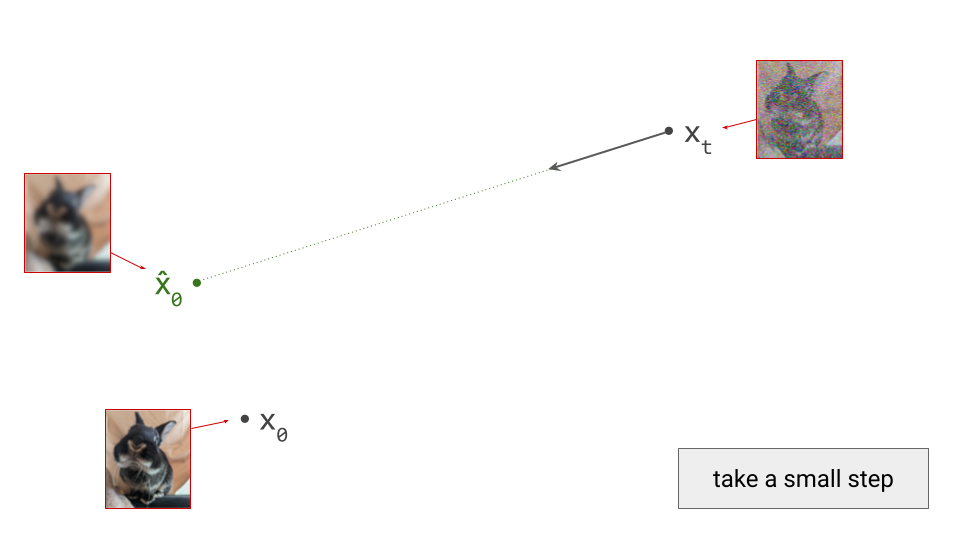
This should look familiar to any machine learning practitioner, as it’s very similar to neural network training via gradient descent: backpropagation gives us the direction of steepest descent at the current point in parameter space, and at each optimisation step, we take a small step in that direction. Taking a very large step wouldn’t get us anywhere interesting, because the estimated direction is only valid locally. The same is true for diffusion sampling, except we’re now operating in the input space, rather than in the space of model parameters.
What happens next depends on the specific sampling algorithm we’ve chosen to use. There are many to choose from: DDPM3 (also called ancestral sampling), DDIM4, DPM++5 and ODE-based sampling6 (with many sub-variants using different ODE solvers) are just a few examples. Some of these algorithms are deterministic, which means the only source of randomness in the sampling procedure is the initial noise on the canvas. Others are stochastic, which means that further noise is injected at each step of the sampling procedure.
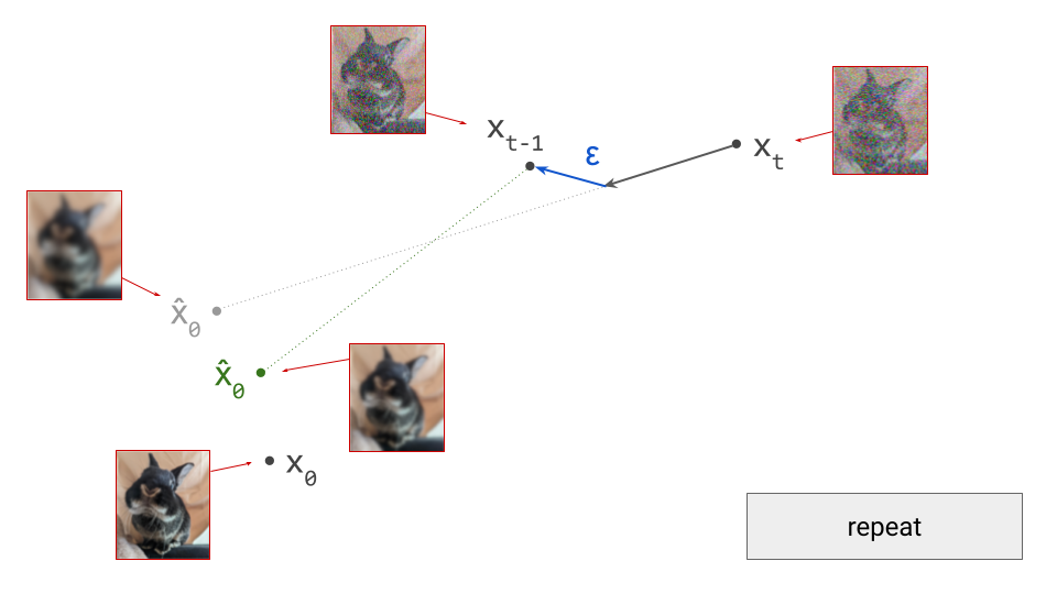
We’ll use DDPM as an example, because it is one of the oldest and most commonly used sampling algorithms for diffusion models. This is a stochastic algorithm, so some random noise is added after taking a step in the direction of the model prediction:
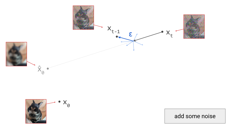
Note that I am intentionally glossing over some of the details of the sampling algorithm here (for example, the exact variance of the noise \(\varepsilon\) that is added at each step). The diagrams are schematic and the focus is on building intuition, so I think I can get away with that, but obviously it’s pretty important to get this right when you actually want to implement this algorithm.
For deterministic sampling algorithms, we can simply skip this step (i.e. set \(\varepsilon = 0\)). After this, we end up in \(\mathbf{x}_{t-1}\), which is the next iterate in the sampling procedure, and should correspond to a slightly less noisy sample. To proceed, we rinse and repeat. We can again make a prediction \(\hat{\mathbf{x}}_0\):
Because we are in a different point in input space, this prediction will also be different. Concretely, as the input to the model is now slightly less noisy, the prediction will be slightly less blurry. We now take a small step in the direction of this new prediction, and add noise to end up in \(\mathbf{x}_{t-2}\):
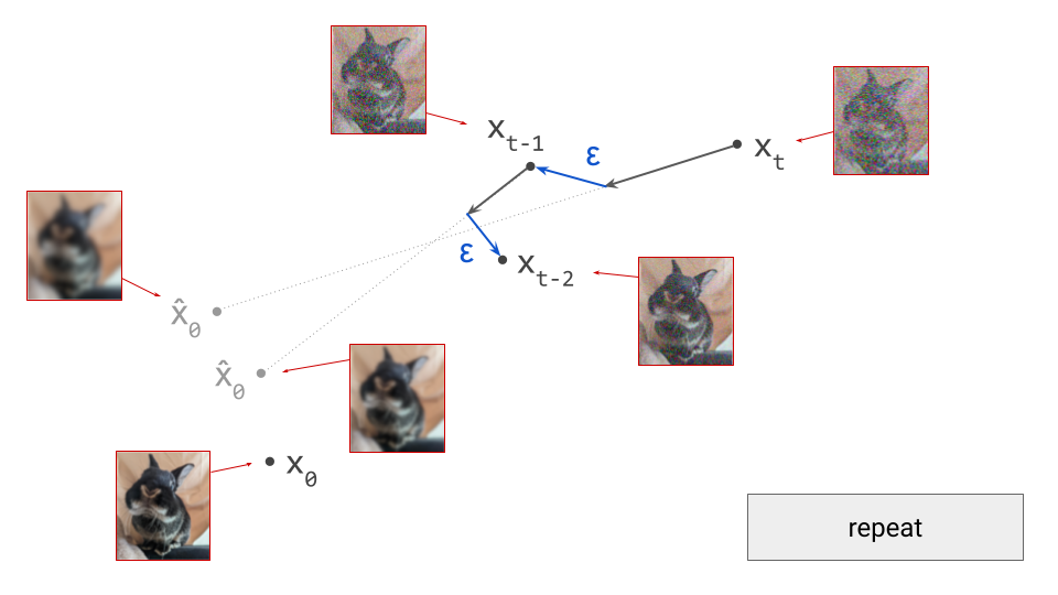
We can keep doing this until we eventually reach \(\mathbf{x}_0\), and we will have drawn a sample from the diffusion model. To summarise, below is an animated version of the above set of diagrams, showing the sequence of steps:

Classifier guidance
Classifier guidance6 7 8 provides a way to steer diffusion sampling in the direction that maximises the probability of the final sample being classified as a particular class. More broadly, this can be used to make the sample reflect any sort of conditioning signal that wasn’t provided to the diffusion model during training. In other words, it enables post-hoc conditioning.
For classifier guidance, we need an auxiliary model that predicts \(p(y \mid \mathbf{x})\), where \(y\) represents an arbitrary input feature, which could be a class label, a textual description of the input, or even a more structured object like a segmentation map or a depth map. We’ll call this model a classifier, but keep in mind that we can use many different kinds of models for this purpose, not just classifiers in the narrow sense of the word. What’s nice about this setup, is that such models are usually smaller and easier to train than diffusion models.
One important caveat is that we will be applying this auxiliary model to noisy inputs \(\mathbf{x}_t\), at varying levels of noise, so it has to be robust against this particular type of input distortion. This seems to preclude the use of off-the-shelf classifiers, and implies that we need to train a custom noise-robust classifier, or at the very least, fine-tune an off-the-shelf classifier to be noise-robust. We can also explicitly condition the classifier on the time step \(t\), so the level of noise does not have to be inferred from the input \(\mathbf{x}_t\) alone.
However, it turns out that we can construct a reasonable noise-robust classifier by combining an off-the-shelf classifier (which expects noise-free inputs) with our diffusion model. Rather than applying the classifier to \(\mathbf{x}_t\), we first predict \(\hat{\mathbf{x}}_0\) with the diffusion model, and use that as input to the classifier instead. \(\hat{\mathbf{x}}_0\) is still distorted, but by blurring rather than by Gaussian noise. Off-the-shelf classifiers tend to be much more robust to this kind of distortion out of the box. Bansal et al.9 named this trick “forward universal guidance”, though it has been known for some time. They also suggest some more advanced approaches for post-hoc guidance.
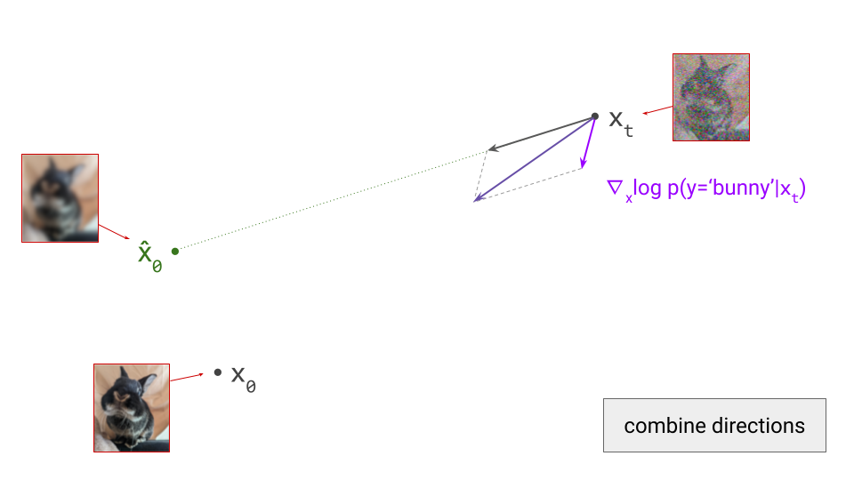
Using the classifier, we can now determine the direction in input space that maximises the log-likelihood of the conditioning signal, simply by computing the gradient with respect to \(\mathbf{x}_t\): \(\nabla_{\mathbf{x}_t} \log p(y \mid \mathbf{x}_t)\). (Note: if we used the above trick to construct a noise-robust classifier from an off-the-shelf one, this means we’ll need to backpropagate through the diffusion model as well.)
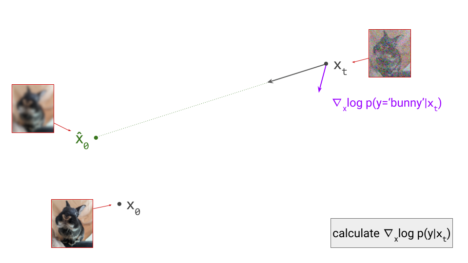
To apply classifier guidance, we combine the directions obtained from the diffusion model and from the classifier by adding them together, and then we take a step in this combined direction instead:
As a result, the sampling procedure will trace a different trajectory through the input space. To control the influence of the conditioning signal on the sampling procedure, we can scale the contribution of the classifier gradient by a factor \(\gamma\), which is called the guidance scale:
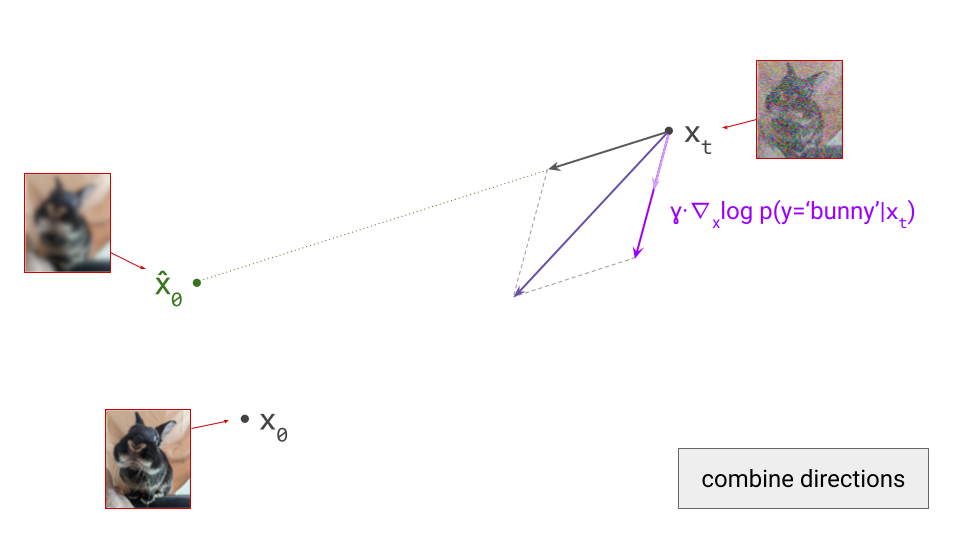
The combined update direction will then be influenced more strongly by the direction obtained from the classifier (provided that \(\gamma > 1\), which is usually the case):
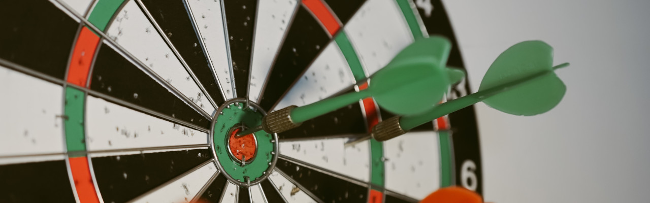
This scale factor \(\gamma\) is an important sampling hyperparameter: if it’s too low, the effect is negligible. If it’s too high, the samples will be distorted and low-quality. This is because gradients obtained from classifiers don’t necessarily point in directions that lie on the image manifold – if we’re not careful, we may actually end up in adversarial examples, which maximise the probability of the class label but don’t actually look like an example of the class at all!
In my previous blog post on diffusion guidance, I made the connection between these operations on vectors in the input space, and the underlying manipulations of distributions they correspond to. It’s worth briefly revisiting this connection to make it more apparent:
-
We’ve taken the update direction obtained from the diffusion model, which corresponds to \(\nabla_{\mathbf{x}_t} \log p_t(\mathbf{x}_t)\) (i.e. the score function), and the (scaled) update direction obtained from the classifier, \(\gamma \cdot \nabla_{\mathbf{x}_t} \log p(y \mid \mathbf{x}_t)\), and combined them simply by adding them together: \(\nabla_{\mathbf{x}_t} \log p_t(\mathbf{x}_t) + \gamma \cdot \nabla_{\mathbf{x}_t} \log p(y \mid \mathbf{x}_t)\).
-
This expression corresponds to the gradient of the logarithm of \(p_t(\mathbf{x}_t) \cdot p(y \mid \mathbf{x}_t)^\gamma\).
-
In other words, we have effectively reweighted the model distribution, changing the probability of each input in accordance with the probability the classifier assigns to the desired class label.
-
The guidance scale \(\gamma\) corresponds to the temperature of the classifier distribution. A high temperature implies that inputs to which the classifier assigns high probabilities are upweighted more aggressively, relative to other inputs.
-
The result is a new model that is much more likely to produce samples that align with the desired class label.
An animated diagram of a single step of sampling with classifier guidance is shown below:
Classifier-free guidance
Classifier-free guidance10 is a variant of guidance that does not require an auxiliary classifier model. Instead, a Bayesian classifier is constructed by combining a conditional and an unconditional generative model.
Concretely, when training a conditional generative model \(p(\mathbf{x}\mid y)\), we can drop out the conditioning \(y\) some percentage of the time (usually 10-20%) so that the same model can also act as an unconditional generative model, \(p(\mathbf{x})\). It turns out that this does not have a detrimental effect on conditional modelling performance. Using Bayes’ rule, we find that \(p(y \mid \mathbf{x}) \propto \frac{p(\mathbf{x}\mid y)}{p(\mathbf{x})}\), which gives us a way to turn our generative model into a classifier.
In diffusion models, we tend to express this in terms of score functions, rather than in terms of probability distributions. Taking the logarithm and then the gradient w.r.t. \(\mathbf{x}\), we get \(\nabla_\mathbf{x} \log p(y \mid \mathbf{x}) = \nabla_\mathbf{x} \log p(\mathbf{x} \mid y) - \nabla_\mathbf{x} \log p(\mathbf{x})\). In other words, to obtain the gradient of the classifier log-likelihood with respect to the input, all we have to do is subtract the unconditional score function from the conditional score function.
Substituting this expression into the formula for the update direction of classifier guidance, we obtain the following:
\[\nabla_{\mathbf{x}_t} \log p_t(\mathbf{x}_t) + \gamma \cdot \nabla_{\mathbf{x}_t} \log p(y \mid \mathbf{x}_t)\] \[= \nabla_{\mathbf{x}_t} \log p_t(\mathbf{x}_t) + \gamma \cdot \left( \nabla_{\mathbf{x}_t} \log p(\mathbf{x}_t \mid y) - \nabla_{\mathbf{x}_t} \log p(\mathbf{x}_t) \right)\] \[= (1 - \gamma) \cdot \nabla_{\mathbf{x}_t} \log p_t(\mathbf{x}_t) + \gamma \cdot \nabla_{\mathbf{x}_t} \log p(\mathbf{x}_t \mid y) .\]The update direction is now a linear combination of the unconditional and conditional score functions. It would be a convex combination if it were the case that \(\gamma \in [0, 1]\), but in practice \(\gamma > 1\) tends to be were the magic happens, so this is merely a barycentric combination. Note that \(\gamma = 0\) reduces to the unconditional case, and \(\gamma = 1\) reduces to the conditional (unguided) case.
How do we make sense of this geometrically? With our hybrid conditional/unconditional model, we can make two predictions \(\hat{\mathbf{x}}_0\). These will be different, because the conditioning information may allow us to make a more accurate prediction:
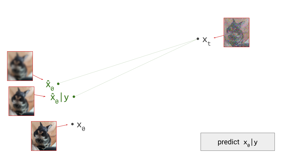
Next, we determine the difference vector between these two predictions. As we showed earlier, this corresponds to the gradient direction provided by the implied Bayesian classifier:

We now scale this vector by \(\gamma\):
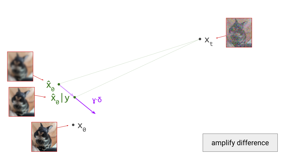
Starting from the unconditional prediction for \(\hat{\mathbf{x}}_0\), this vector points towards a new implicit prediction, which corresponds to a stronger influence of the conditioning signal. This is the prediction we will now take a small step towards:
Classifier-free guidance tends to work a lot better than classifier guidance, because the Bayesian classifier is much more robust than a separately trained one, and the resulting update directions are much less likely to be adversarial. On top of that, it doesn’t require an auxiliary model, and generative models can be made compatible with classifier-free guidance simply through conditioning dropout during training. On the flip side, that means we can’t use this for post-hoc conditioning – all conditioning signals have to be available during training of the generative model itself. My previous blog post on guidance covers the differences in more detail.
An animated diagram of a single step of sampling with classifier-free guidance is shown below:

Closing thoughts
What’s surprising about guidance, in my opinion, is how powerful it is in practice, despite its relative simplicity. The modifications to the sampling procedure required to apply guidance are all linear operations on vectors in the input space. This is what makes it possible to interpret the procedure geometrically.
How can a set of linear operations affect the outcome of the sampling procedure so profoundly? The key is iterative refinement: these simple modifications are applied repeatedly, and crucially, they are interleaved with a very non-linear operation, which is the application of the diffusion model itself, to predict the next update direction. As a result, any linear modification of the update direction has a non-linear effect on the next update direction. Across many sampling steps, the resulting effect is highly non-linear and powerful: small differences in each step accumulate, and result in trajectories with very different endpoints.
I hope the visualisations in this post are a useful complement to my previous writing on the topic of guidance. Feel free to let me know your thoughts in the comments, or on Twitter/X (@sedielem) or Threads (@sanderdieleman).
If you would like to cite this post in an academic context, you can use this BibTeX snippet:
@misc{dieleman2023geometry,
  author = {Dieleman, Sander},
  title = {The geometry of diffusion guidance},
  url = {https://sander.ai/2023/08/28/geometry.html},
  year = {2023}
}
Acknowledgements
Thanks to Bundle for modelling and to kipply for permission to use this photograph. Thanks to my colleagues at Google DeepMind for various discussions, which continue to shape my thoughts on this topic!
References
-
Blum, Hopcroft, Kannan, “Foundations of Data science”, Cambridge University Press, 2020 ↩
-
Song, Dhariwal, Chen, Sutskever, “Consistency Models”, International Conference on Machine Learning, 2023. ↩
-
Ho, Jain, Abbeel, “Denoising Diffusion Probabilistic Models”, 2020. ↩
-
Song, Meng, Ermon, “Denoising Diffusion Implicit Models”, International Conference on Learning Representations, 2021. ↩
-
Lu, Zhou, Bao, Chen, Li, Zhu, “DPM-Solver++: Fast Solver for Guided Sampling of Diffusion Probabilistic Models”, arXiv, 2022. ↩
-
Song, Sohl-Dickstein, Kingma, Kumar, Ermon and Poole, “Score-Based Generative Modeling through Stochastic Differential Equations”, International Conference on Learning Representations, 2021. ↩ ↩2
-
Sohl-Dickstein, Weiss, Maheswaranathan and Ganguli, “Deep Unsupervised Learning using Nonequilibrium Thermodynamics”, International Conference on Machine Learning, 2015. ↩
-
Dhariwal, Nichol, “Diffusion Models Beat GANs on Image Synthesis”, Neural Information Processing Systems, 2021. ↩
-
Bansal, Chu, Schwarzschild, Sengupta, Goldblum, Geiping, Goldstein, “Universal Guidance for Diffusion Models”, Computer Vision and Pattern Recognition, 2023. ↩
-
Ho, Salimans, “Classifier-Free Diffusion Guidance”, NeurIPS workshop on DGMs and Applications”, 2021. ↩