This post is an addendum to my blog post about typicality. Please consider reading that first, if you haven’t already. Here, I will try to quantify what happens when our intuitions fail us in high-dimensional spaces.
Note that the practical relevance of this is limited, so consider this a piece of optional extra content!
In the ‘unfair coin flips’ example from the main blog post, it’s actually pretty clear what happens when our intuitions fail us: we think of the binomial distribution, ignoring the order of the sequences as a factor, when we should actually be taking it into account. Referring back to the table from section 2.1, we use the probabilities in the rightmost column, when we should be using those in the third column. But when we think of a high-dimensional Gaussian distribution and come to the wrong conclusion, what distribution are we actually thinking of?
The Gaussian distribution \(\mathcal{N}_K\)

Let’s start by quantifying what a multivariate Gaussian distribution actually looks like: let \(\mathbf{x} \sim \mathcal{N}(\mathbf{0}, I_K)\), a standard Gaussian distribution in \(K\) dimensions, henceforth referred to as \(\mathcal{N}_K\). We can sample from it by drawing \(K\) independent one-dimensional samples \(x_i \sim \mathcal{N}(0, 1)\), and joining them into a vector \(\mathbf{x}\). This distribution is spherically symmetric, which makes it very natural to think about samples in terms of their distance to the mode (in this case, the origin, corresponding to the zero-vector \(\mathbf{0}\)), because all samples at a given distance \(r\) have the same density.
Now, let’s look at the distribution of \(r\): it seems as if the multivariate Gaussian distribution \(\mathcal{N}_K\) naturally arises by taking a univariate version of it, and rotating it around the mode in every possible direction in \(K\)-dimensional space. Because each of these individual rotated copies is Gaussian, this in turn might seem to imply that the distance from the mode \(r\) is itself Gaussian (or rather half-Gaussian, since it is a nonnegative quantity). But this is incorrect! \(r\) actually follows a chi distribution with \(K\) degrees of freedom: \(r \sim \chi_K\).
Note that for \(K = 1\), this does indeed correspond to a half-Gaussian distribution. But as \(K\) increases, the mode of the chi distribution rapidly shifts away from 0: it actually sits at \(\sqrt{K - 1}\). This leaves considerably less probability mass near 0, where the mode of our original multivariate Gaussian \(\mathcal{N}_K\) is located.
This exercise yields an alternative sampling strategy for multivariate Gaussians: first, sample a distance from the mode \(r \sim \chi_K\). Then, sample a direction, i.e. a vector on the \(K\)-dimensional unit sphere \(S^K\), uniformly at random: \(\mathbf{\theta} \sim U[S^K]\). Multiply them together to obtain a Gaussian sample: \(\mathbf{x} = r \cdot \mathbf{\theta} \sim \mathcal{N}_K\).
The Gaussian mirage distribution \(\mathcal{M}_K\)

What if, instead of sampling \(r \sim \chi_K\), we sampled \(r \sim \mathcal{N}(0, K)\) instead? Note that \(\sigma^2_{\chi_K} = K\), so this change preserves the scale of the resulting vectors. For \(K = 1\), we get the same distribution for \(\mathbf{x}\), but for \(K > 1\), we get something very different. The resulting distribution represents what we might think the multivariate Gaussian distribution looks like, if we rely on a mistaken intuition and squint a bit. Let’s call this the Gaussian mirage distribution, denoted by \(\mathcal{M}\): \(\mathbf{x} = r \cdot \mathbf{\theta} \sim \mathcal{M}_K\). (If this thing already has a name, I’m not aware of it, so please let me know!)
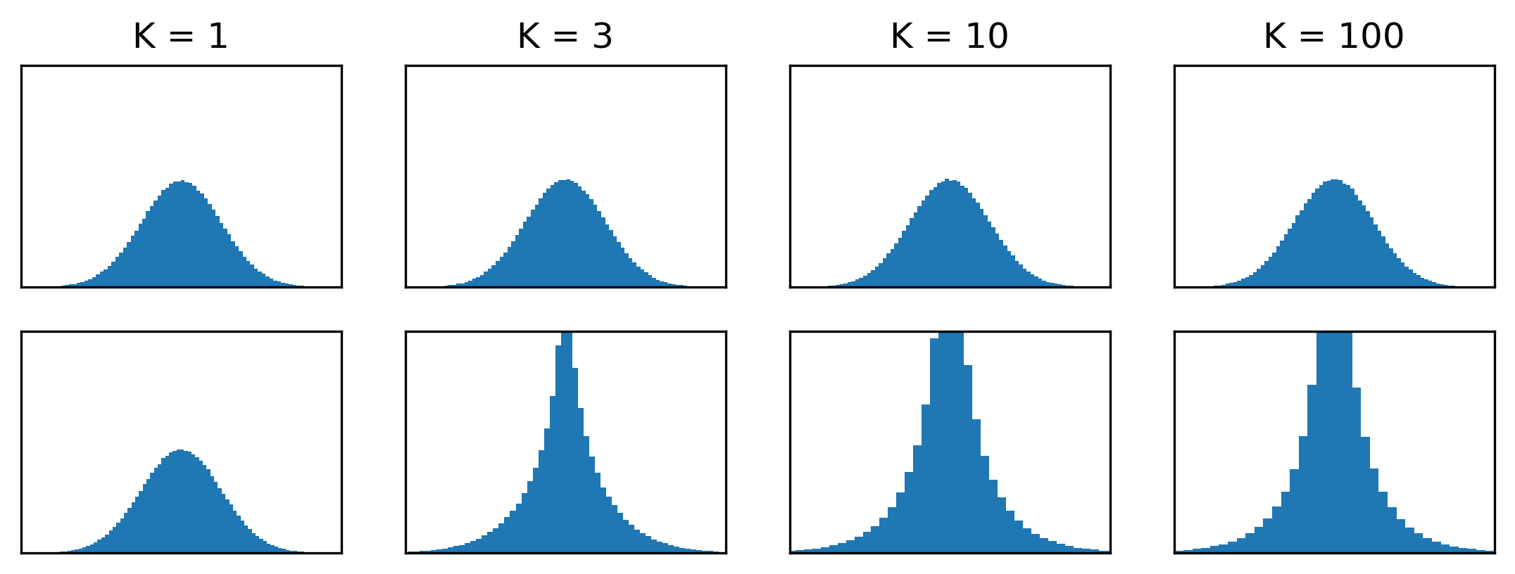
We’ve already established that \(\mathcal{M}_1 \equiv \mathcal{N}_1\). But in higher dimensions, these distributions behave very differently. One way to comprehend this is to look at a flattened histogram of samples across all coordinates:
import matplotlib.pyplot as plt
import numpy as np

def gaussian(n, k):
    return np.random.normal(0, 1, (n, k))

def mirage(n, k):
    direction = np.random.normal(0, 1, (n, k))
    direction /= np.sqrt(np.sum(direction**2, axis=-1, keepdims=True))
    distance = np.random.normal(0, np.sqrt(k), (n, 1))
    return distance * direction

def plot_histogram(x):
    plt.hist(x.ravel(), bins=100)
    plt.ylim(0, 80000)
    plt.xlim(-4, 4)
    plt.tick_params(labelleft=False, left=False, labelbottom=False, bottom=False)

plt.figure(figsize=(9, 3))
ks = [1, 3, 10, 100]
for i, k in enumerate(ks):
    plt.subplot(2, len(ks), i + 1)
    plt.title(f'K = {k}')
    plot_histogram(gaussian(10**6 // k, k))
    plt.subplot(2, len(ks), i + 1 + len(ks))
    plot_histogram(mirage(10**6 // k, k))

For \(\mathcal{N}_K\), this predictably looks like a univariate Gaussian for all \(K\). For \(\mathcal{M}_K\), it becomes highly leptokurtic as \(K\) increases, indicating that dramatically more probability mass is located close to the mode.
Typical sets of \(\mathcal{N}_K\) and \(\mathcal{M}_K\)
Let’s also look at the typical sets for both of these distributions. For \(\mathcal{N}_K\), the probability density function (pdf) has the form:
\[f_{\mathcal{N}_K}(\mathbf{x}) = (2 \pi)^{-\frac{K}{2}} \exp \left( -\frac{\mathbf{x}^T \mathbf{x}}{2} \right),\]and the differential entropy is given by:
\[H_{\mathcal{N}_K} = \frac{K}{2} \log \left(2 \pi e \right) .\]To find the typical set, we just need to look for the \(\mathbf{x}\) where \(f_{\mathcal{N}_K}(\mathbf{x}) \approx 2^{-H_{\mathcal{N}_K}} = (2 \pi e)^{-\frac{K}{2}}\) (assuming the entropy is measured in bits). This is clearly the case when \(\mathbf{x}^T\mathbf{x} \approx K\), or in other words, for any \(\mathbf{x}\) whose distance from the mode is close to \(\sqrt{K}\). This is the Gaussian annulus from before.
Let’s subject the Gaussian mirage \(\mathcal{M}_K\) to the same treatment. It’s not obvious how to express the pdf in terms of \(\mathbf{x}\), but it’s easier if we rewrite \(\mathbf{x}\) as \(r \cdot \mathbf{\theta}\), as before, and imagine the sampling procedure: first, pick a radius \(r \sim \mathcal{HN}(0, K)\) (the half-Gaussian distribution — using the Gaussian distribution complicates the math a bit, because the radius should be nonnegative), and then pick a position on the \(K\)-sphere with radius \(r\), uniformly at random:
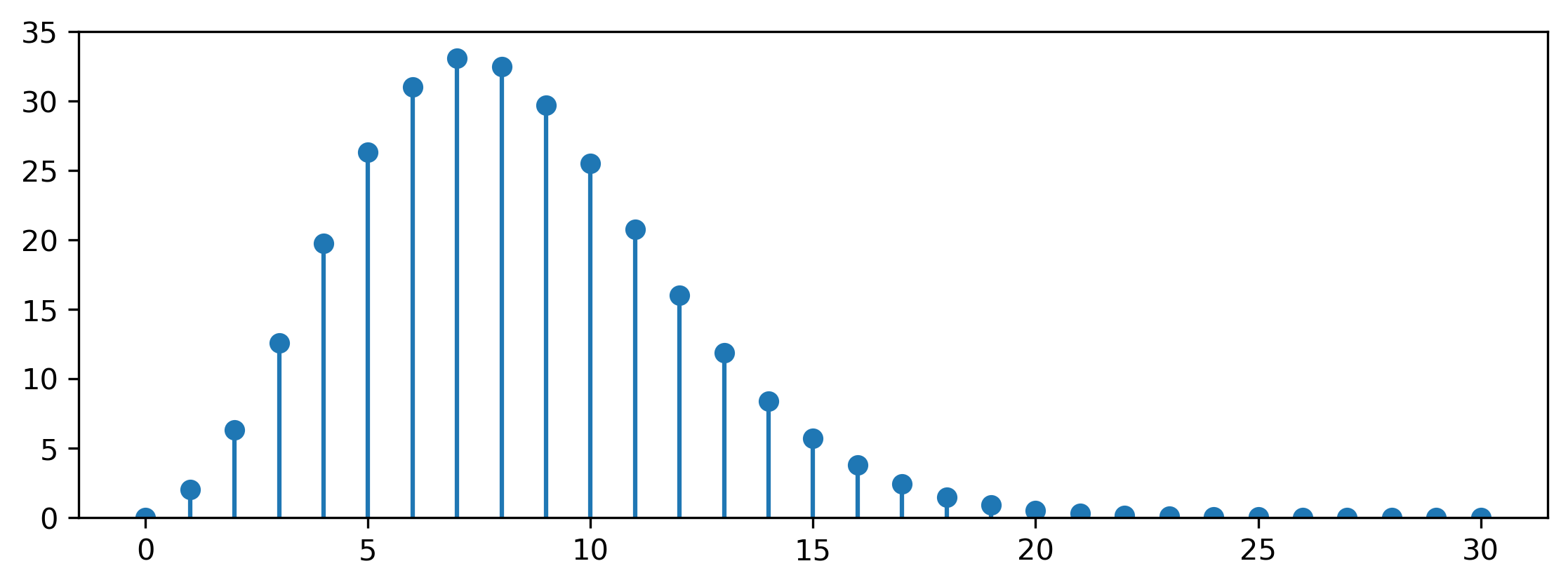
\[f_{\mathcal{M}_K}(\mathbf{x}) = f_{\mathcal{HN}(0, K)}(r) \cdot f_{U[S^K(r)]}(\theta) = \frac{2}{\sqrt{2 \pi K}} \exp \left( -\frac{r^2}{2 K} \right) \cdot \frac{1}{r^{K-1}} \frac{\Gamma\left( \frac{K}{2} \right)}{2 \pi ^ \frac{K}{2}} .\]The former factor is the density of the half-Gaussian distribution: note the additional factor 2 compared to the standard Gaussian density, because we only consider nonnegative values of \(r\). The latter is the density of a uniform distribution on the \(K\)-sphere with radius \(r\) (which is the inverse of its surface area). As an aside, this factor is worth taking a closer look at, because it behaves in a rather peculiar way. Here’s the surface area of a unit \(K\)-sphere for increasing \(K\):
import matplotlib.pyplot as plt
import numpy as np
import scipy.special

K = np.arange(0, 30 + 1)
A = (2 * np.pi**(K / 2.0)) / scipy.special.gamma(K / 2.0)
plt.figure(figsize=(9, 3))
plt.stem(K, A, basefmt=' ')
plt.ylim(0, 35)

Confused? You and me both! Believe it or not, the surface area of a \(K\)-sphere tends to zero with increasing \(K\) — but only after growing to a maximum at \(K = 7\) first. High-dimensional spaces are weird.
Another thing worth noting is that the density at the mode \(f_{\mathcal{M}_K}(\mathbf{0}) = +\infty\) for \(K > 1\), which already suggests that this distribution has a lot of its mass concentrated near the mode.
Computing the entropy of this distribution takes a bit of work. The differential entropy is:
\[H_{\mathcal{M}_K} = - \int_{\mathbb{R}^K} f_{\mathcal{M}_K}(\mathbf{x}) \log f_{\mathcal{M}_K}(\mathbf{x}) \mathrm{d}\mathbf{x} .\]We can use the radial symmetry of this density to reformulate this as an integral of a scalar function:
\[H_{\mathcal{M}_K} = - \int_0^{+\infty} f_{\mathcal{M}_K}(r) \log f_{\mathcal{M}_K}(r) S^K(r) \mathrm{d} r,\]where \(S^K(r)\) is the surface area of a \(K\)-sphere with radius \(r\). Filling in the density function, we get:
\[H_{\mathcal{M}_K} = - \int_0^{+\infty} \frac{2}{\sqrt{2 \pi K}} \exp \left( -\frac{r^2}{2 K} \right) \cdot \log \left( \frac{2}{\sqrt{2 \pi K}} \exp \left( -\frac{r^2}{2 K} \right) \cdot \frac{1}{r^{K-1}} \frac{\Gamma\left( \frac{K}{2} \right)}{2 \pi ^ \frac{K}{2}} \right) \mathrm{d} r,\]where we have made use of the fact that \(S^K(r)\) cancels out with the second factor of \(f_{\mathcal{M}_K}(r)\). We can split up the \(\log\) into three different terms, \(H_{\mathcal{M}_K} = H_1 + H_2 + H_3\):
\[H_1 = - \int_0^{+\infty} \frac{2}{\sqrt{2 \pi K}} \exp \left( -\frac{r^2}{2 K} \right) \left(-\frac{r^2}{2 K} \right) \mathrm{d} r = \int_0^{+\infty} \frac{r^2}{\sqrt{2 \pi}} \exp \left( -\frac{r^2}{2} \right) \mathrm{d} r = \frac{1}{2},\] \[H_2 = - \int_0^{+\infty} \frac{2}{\sqrt{2 \pi K}} \exp \left( -\frac{r^2}{2 K} \right) \log \left( \frac{1}{r^{K-1}} \right) \mathrm{d} r = \frac{K - 1}{2} \left( \log \frac{K}{2} - \gamma \right),\] \[H_3 = - \int_0^{+\infty} \frac{2}{\sqrt{2 \pi K}} \exp \left( -\frac{r^2}{2 K} \right) \log \left( \frac{2}{\sqrt{2 \pi K}} \frac{\Gamma\left( \frac{K}{2} \right)}{2 \pi ^ \frac{K}{2}} \right) \mathrm{d} r = - \log \left( \frac{1}{\sqrt{2 \pi K}} \frac{\Gamma\left( \frac{K}{2} \right)}{\pi ^ \frac{K}{2}} \right),\]where we have taken \(\log\) to be the natural logarithm for convenience, and \(\gamma\) is the Euler-Mascheroni constant. In summary:
\[H_{\mathcal{M}_K} = \frac{1}{2} + \frac{K - 1}{2} \left( \log \frac{K}{2} - \gamma \right) - \log \left( \frac{1}{\sqrt{2 \pi K}} \frac{\Gamma\left( \frac{K}{2} \right)}{\pi ^ \frac{K}{2}} \right) .\]Note that \(H_{\mathcal{M}_1} = \frac{1}{2} \log (2 \pi e)\), matching the standard Gaussian distribution as expected.
Because this is measured in nats, not in bits, we find the typical set where \(f_{\mathcal{M}_K}(\mathbf{x}) \approx \exp(-H_{\mathcal{M}_K})\). We must find \(r \geq 0\) so that
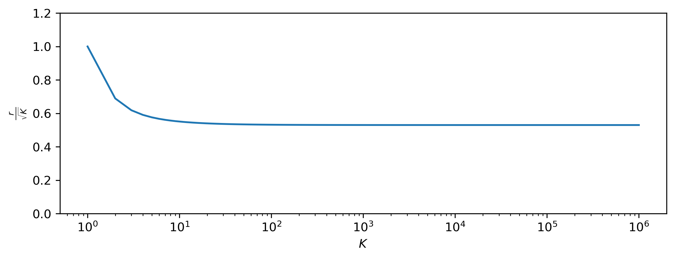
\[\frac{r^2}{2 K} + (K - 1) \log r = \frac{1}{2} + \frac{K - 1}{2} \left( \log \frac{K}{2} - \gamma \right) .\]We can express the solution of this equation in terms of the Lambert \(W\) function:
\[r = \sqrt{K (K - 1) W\left(\frac{1}{K (K - 1)} \exp \left( \frac{1}{K - 1} + \log \frac{K}{2} - \gamma \right) \right)} .\]import matplotlib.pyplot as plt
import numpy as np
import scipy.special
K = np.unique(np.round(np.logspace(0, 6, 100)))
w_arg = np.exp(1 / (K - 1) + np.log(K / 2) - np.euler_gamma) / (K * (K - 1))
r = np.sqrt(K * (K - 1) * scipy.special.lambertw(w_arg))
r[0] = 1 # Special case for K = 1.
plt.figure(figsize=(9, 3))
plt.plot(K, r / np.sqrt(K))
plt.xscale('log')
plt.ylim(0, 1.2)
plt.xlabel('$K$')
plt.ylabel('$\\frac{r}{\\sqrt{K}}$')

As \(K \to +\infty\), this seems to converge to the value \(0.52984 \sqrt{K}\), which is somewhere in between the mode (\(0\)) and the mean (\(\sqrt{\frac{2K}{\pi}} \approx 0.79788 \sqrt{K}\)) of the half-Gaussian distribution (which \(r\) follows by construction). This is not just an interesting curiosity: although it is clear that the typical set of \(\mathcal{M}_K\) is much closer to the mode than for \(\mathcal{N}_K\) (because \(r < \sqrt{K}\)), the mode is not unequivocally a member of the typical set. In fact, the definition of typical sets sort of breaks down for this distribution, because we need to allow for a very large range of probability densities to capture the bulk of its mass. In this sense, it behaves a lot more like the one-dimensional Gaussian. Nevertheless, even this strange concoction of a distribution exhibits unintuitive behaviour in high-dimensional space!
If you would like to cite this post in an academic context, you can use this BibTeX snippet:
@misc{dieleman2020typicality,
  author = {Dieleman, Sander},
  title = {Musings on typicality},
  url = {https://benanne.github.io/2020/09/01/typicality.html},
  year = {2020}
}
