Most contemporary generative models of images, sound and video do not operate directly on pixels or waveforms. They consist of two stages: first, a compact, higher-level latent representation is extracted, and then an iterative generative process operates on this representation instead. How does this work, and why is this approach so popular?
Generative models that make use of latent representations are everywhere nowadays, so I thought it was high time to dedicate a blog post to them. In what follows, I will talk at length about latents as a plural noun, which is the usual shorthand for latent representation. This terminology originated in the concept of latent variables in statistics, but it is worth noting that the meaning has drifted somewhat in this context. These latents do not represent any known underlying physical quantity which we cannot measure directly; rather, they capture perceptually meaningful information in a compact way, and in many cases they are a deterministic nonlinear function of the input signal (i.e. not random variables).
In what follows, I will assume a basic understanding of neural networks, generative models and related concepts. Below is an overview of the different sections of this post. Click to jump directly to a particular section.
- The recipe
- How we got here
- Why two stages?
- Trading off reconstruction quality and modelability
- Controlling capacity
- Curating and shaping the latent space
- The tyranny of the grid
- Latents for other modalities
- Will end-to-end win in the end?
- Closing thoughts
- Acknowledgements
- References
The recipe
The usual process for training a generative model in latent space consists of two stages:
- Train an autoencoder on the input signals. This is a neural network consisting of two subnetworks, an encoder and a decoder. The former maps an input signal to its corresponding latent representation (encoding). The latter maps the latent representation back to the input domain (decoding).
- Train a generative model on the latent representations. This involves taking the encoder from the first stage, and using it to extract latents for the training data. The generative model is then trained directly on these latents. Nowadays, this is usually either an autoregressive model or a diffusion model.
Once the autoencoder is trained in the first stage, its parameters will not change any further in the second stage: gradients from the second stage of the learning process are not backpropagated into the encoder. Another way to say this is that the encoder parameters are frozen in the second stage.
Note that the decoder part of the autoencoder plays no role in the second stage of training, but we will need it when sampling from the generative model, as that will generate outputs in latent space. The decoder enables us to map the generated latents back to the original input space.
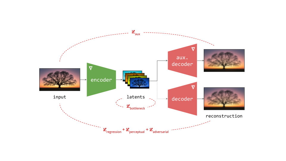
Below is a diagram illustrating this two-stage training recipe. Networks whose parameters are learnt in the respective stages are indicated with a \(\nabla\) symbol, because this is almost always done using gradient-based learning. Networks whose parameters are frozen are indicated with a snowflake.
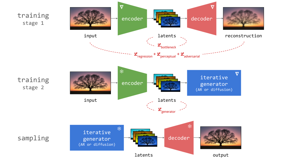
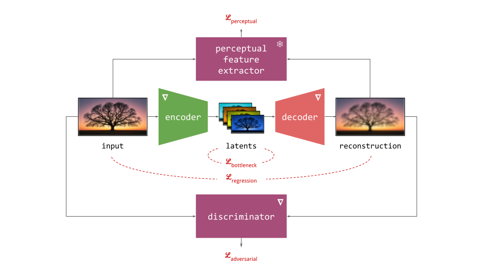
Several different loss functions are involved in the two training stages, which are indicated in red on the diagram:
- To ensure the encoder and decoder are able to convert input representations to latents and back with high fidelity, several loss functions constrain the reconstruction (decoder output) with respect to the input. These usualy include a simple regression loss, a perceptual loss and an adversarial loss.
- To constrain the capacity of the latents, an additional loss function is often applied directly to them during training, although this is not always the case. We will refer to this as the bottleneck loss, because the latent representation forms a bottleneck in the autoencoder network.
- In the second stage, the generative model is trained using its own loss function, separate from those used during the first stage. This is often the negative log-likelihood loss (for autoregressive models), or a diffusion loss.
Taking a closer look at the reconstruction-based losses, we have:
- the regression loss, which is sometimes the mean absolute error (MAE) measured in the input space (e.g. on pixels), but more often the mean squared error (MSE).
- the perceptual loss, which can take many forms, but more often than not, it makes use of another frozen pre-trained neural network to extract perceptual features. The loss encourages these features to match between the reconstruction and the input, which results in better preservation of high-frequency content that is largely ignored by the regression loss. LPIPS1 is a popular choice for images.
- the adversarial loss, which uses a discriminator network which is co-trained with the autoencoder, as in generative adversarial networks (GANs)2. The discriminator is trained to tell apart real input signals from reconstructions, and the autoencoder is trained to fool the discriminator into making mistakes. The goal is to improve the realism of the output, even if it means deviating further from the input signal. It is quite common for the adversarial loss to be disabled for some time at the start of training, to avoid instability.
Below is a more elaborate diagram of the first training stage, explicitly showing the other networks which typically play a role in this process.
It goes without saying that this generic recipe is often deviated from in one or more ways, especially for audio and video, but I have tried to summarise the most common ingredients found in most modern practical applications of this modelling approach.
How we got here
The two dominant generative modelling paradigms of today, autoregression and diffusion, were both initially applied to “raw” digital representations of perceptual signals, by which I mean pixels and waveforms. PixelRNN3 and PixelCNN4 generated images one pixel at a time. WaveNet5 and SampleRNN6 did the same for audio, producing waveform amplitudes one sample at a time. On the diffusion side, the original works that introduced7 and established8 9 the modelling paradigm all operated on pixels to produce images, and early works like WaveGrad10 and DiffWave11 generated waveforms to produce sound.
However, it became clear very quickly that this strategy makes scaling up quite challenging. The most important reason for this can be summarised as follows: perceptual signals mostly consist of imperceptible noise. Or, to put it a different way: out of the total information content of a given signal, only a small fraction actually affects our perception of it. Therefore, it pays to ensure that our generative model can use its capacity efficiently, and focus on modelling just that fraction. That way, we can use smaller, faster and cheaper generative models without compromising on perceptual quality.
Latent autoregression
Autoregressive models of images took a huge leap forward with the seminal VQ-VAE paper12. It suggested a practical strategy for learning discrete representations with neural networks, by inserting a vector quantisation bottleneck layer into an autoencoder. To learn such discrete latents for images, a convolutional encoder with several downsampling stages produced a spatial grid of vectors with a 4× lower resolution than the input (along both height and width, so 16× fewer spatial positions), and these vectors were then quantised by the bottleneck layer.
Now, we could generate images with PixelCNN-style models one latent vector at a time, rather than having to do it pixel by pixel. This significantly reduced the number of autoregressive sampling steps required, but perhaps more importantly, measuring the likelihood loss in the latent space rather than pixel space helped avoid wasting capacity on imperceptible noise. This is effectively a different loss function, putting more weight on perceptually relevant signal content, because a lot of the perceptually irrelevant signal content is not present in the latent vectors (see my blog post on typicality for more on this topic). The paper showed 128×128 generated images from a model trained on ImageNet, a resolution that had only been attainable with GANs2 up to that point.
The discretisation was critical to its success, because autoregressive models were known to work much better with discrete inputs at the time. But perhaps even more importantly, the spatial structure of the latents allowed existing pixel-based models to be adapted very easily. Before this, VAEs (variational autoencoders13 14) would typically compress an entire image into a single latent vector, resulting in a representation without any kind of topological structure. The grid structure of modern latent representations, which mirrors that of the “raw” input representation, is exploited in the network architecture of generative models to increase efficiency (through e.g. convolutions, recurrence or attention layers).
VQ-VAE 215 further increased the resolution to 256x256 and dramatically improved image quality through scale, as well as the use of multiple levels of latent grids, structured in a hierarchy. This was followed by VQGAN16, which combined the adversarial learning mechanism of GANs with the VQ-VAE architecture. This enabled a dramatic increase of the resolution reduction factor from 4× to 16× (256× fewer spatial positions compared to pixel input), while still allowing for sharp and realistic reconstructions. The adversarial loss played a big role in this, encouraging realistic decoder output even when it is not possible to closely adhere to the original input signal.
VQGAN became a core technology enabling the rapid progress in generative modelling of perceptual signals that we’ve witnessed in the last five years. Its impact cannot be overestimated – I’ve gone as far as to say that it’s probably the main reason why GANs deserved to win the Test of Time award at NeurIPS 2024. The “assist” that the VQGAN paper provided, kept GANs relevant even after they were all but replaced by diffusion models for the base task of media generation.
IMO VQGAN is why GANs deserve the NeurIPS test of time award. Suddenly our image representations were an order of magnitude more compact. Absolute game changer for generative modelling at scale, and the basis for latent diffusion models.https://t.co/Ochh17IvGx
— Sander Dieleman (@sedielem) November 28, 2024
It is also worth pointing out just how much of the recipe from the previous section was conceived in this paper. The iterative generator isn’t usually autoregressive these days (Parti17, xAI’s recent Aurora model and, apparently, OpenAI’s GPT-4o are notable exceptions), and the quantisation bottleneck has been replaced, but everything else is still there. Especially the combination of a simple regression loss, a perceptual loss and an adversarial loss has stubbornly persisted, in spite of its apparent complexity. This kind of endurance is rare in a fast-moving field like machine learning – perhaps rivalled only by that of the largely unchanged Transformer architecture18 and the Adam optimiser19!
(While discrete representations played an essential role in making latent autoregression work at scale, I wanted to point out that autoregression in continuous space has also been made to work well recently20 21.)
Latent diffusion
With latent autoregression gaining ground in the late 2010s, and diffusion models breaking through in the early 2020s, combining the strengths of both approaches was a natural next step. As with many ideas whose time has come, we saw a string of concurrent papers exploring this topic hit arXiv around the same time, in the second half of 202122 23 24 25 26. The most well-known of these is Rombach et al.’s High-Resolution Image Synthesis with Latent Diffusion Models26, who reused their previous VQGAN work16 and swapped out the autoregressive Transformer for a UNet-based diffusion model. This formed the basis for the Stable Diffusion models. Other works explored similar ideas, albeit at a smaller scale24, or for modalities other than images22.
It took a little bit of time for the approach to become mainstream. Early commercial text-to-image models made use of so-called resolution cascades, consisting of a base diffusion model that generates low-resolution images directly in pixel space, and one or more upsampling diffusion models that produce higher-resolution outputs conditioned on lower-resolution inputs. Examples include DALL-E 2 and Imagen 2. After Stable Diffusion, most moved to a latent-based approach (including DALL-E 3 and Imagen 3).
An important difference between autoregressive and diffusion models is the loss function used to train them. In the autoregressive case, things are relatively simple: you just maximise the likelihood (although other things have been tried as well27). For diffusion, things are a little more interesting: the loss is an expectation over all noise levels, and the relative weighting of these noise levels significantly affects what the model learns (for an explanation of this, see my previous blog post on noise schedules, as well as my blog post about casting diffusion as autoregression in frequency space). This justifies an interpretation of the typical diffusion loss as a kind of perceptual loss function, which puts more emphasis on signal content that is more perceptually salient.
At first glance, this makes the two-stage approach seem redundant, as it operates in a similar way, i.e. filtering out perceptually irrelevant signal content, to avoid wasting model capacity on it. If we can rely on the diffusion loss to focus only on what matters perceptually, why do we need a separate representation learning stage to filter out the stuff that doesn’t? These two mechanisms turn out to be quite complementary in practice however, for two reasons:
- The way perception works at small and large scales, especially in the visual domain, seems to be fundamentally different – to the extent that modelling texture and fine-grained detail merits separate treatment, and an adversarial approach can be more suitable for this. I will discuss this in more detail in the next section.
- Training large, powerful diffusion models is inherently computationally intensive, and operating in a more compact latent space allows us to avoid having to work with bulky input representations. This helps to reduce memory requirements and speeds up training and sampling.
Some early works did consider an end-to-end approach, jointly learning the latent representation and the diffusion prior23 25, but this didn’t really catch on. Although avoiding sequential dependencies between multiple stages of training is desirable from a practical perspective, the perceptual and computational benefits make it worth the hassle.
Why two stages?
As discussed before, it is important to ensure that generative models of perceptual signals can use their capacity efficiently, as this makes them much more cost-effective. This is essentially what the two-stage approach accomplishes: by extracting a more compact representation that focuses on the perceptually relevant fraction of signal content, and modelling that instead of the original representation, we are able to make relatively modestly sized generative models punch above their weight.
The fact that most bits of information in perceptual signals don’t actually matter perceptually is hardly a new observation: it is also the key idea underlying lossy compression, which enables us to store and transmit these signals at a fraction of the cost. Compression algorithms like JPEG and MP3 exploit the redundancies present in signals, as well as the fact that our audiovisual senses are more sensitive to low frequencies than to high frequencies, to represent perceptual signals with far fewer bits. (There are other perceptual effects that play a role, such as auditory masking for example, but non-uniform frequency sensitivity is the most important one.)
So why don’t we use these lossy compression techniques as a basis for our generative models then? This is not a bad idea, and several works have used these algorithms, or parts of them, for this purpose28 29 30. But a very natural reflex for people working on generative models is to try to solve the problem with more machine learning, to see if we can do better than these “handcrafted” algorithms.
It’s not just hubris on the part of ML researchers, though: there is actually a very good reason to use learned latents, instead of using these pre-existing compressed representations. Unlike in the compression setting, where smaller is better, and size is all that matters, the goal of generative modelling also imposes other constraints: some representations are easier to model than others. It is crucial that some structure remains in the representation, which we can then exploit by endowing the generative model with the appropriate inductive biases. This requirement creates a trade-off between reconstruction quality and modelability of the latents, which we will investigate in the next section.
An important reason behind the efficacy of latent representations is how they lean in to the fact that our perception works differently at different scales. In the audio domain, this is readily apparent: very rapid changes in amplitude result in the perception of pitch, whereas changes on coarser time scales (e.g. drum beats) can be individually discerned. Less well-known is that the same phenomenon also plays an important role in visual perception: rapid local fluctuations in colour and intensity are perceived as textures. A while back, I tried to explain this on Twitter, and I will paraphrase that explanation here:
One way to think of it is texture vs. structure, or sometimes people call this stuff vs. things.
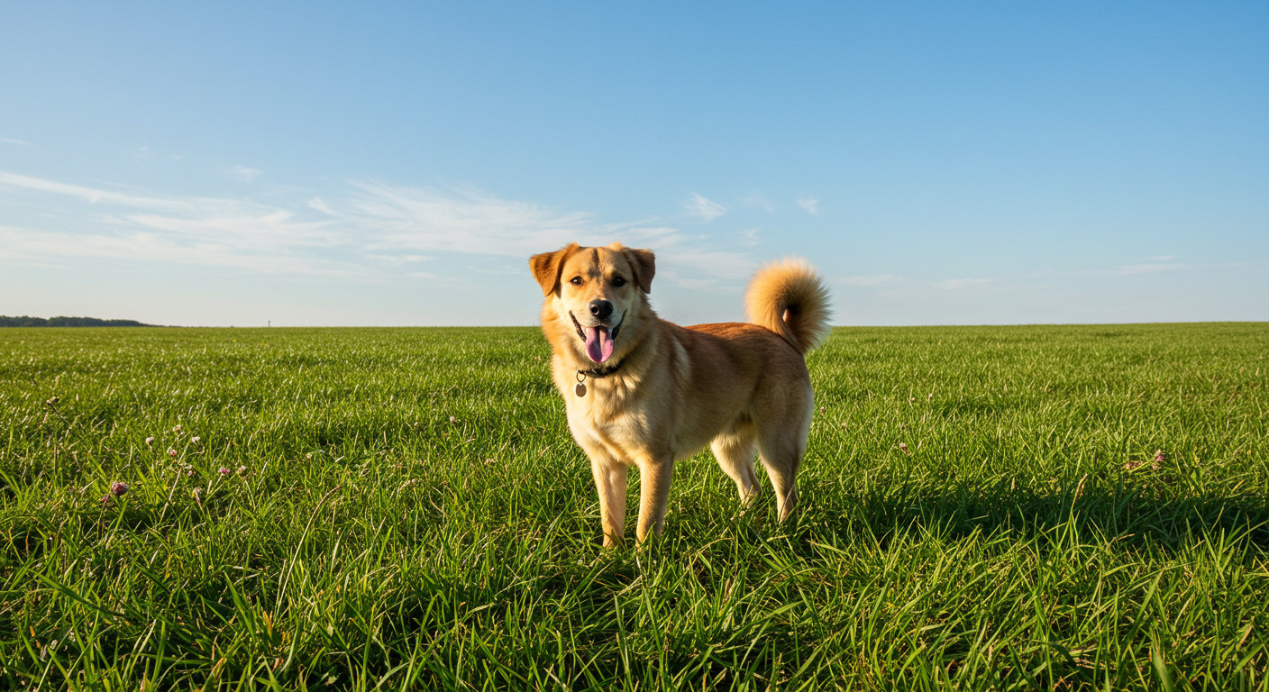
In an image of a dog in a field, the grass texture (stuff) is high-entropy, but we are bad at perceiving differences between individual realisations of this texture, we just perceive it as "grass", in an uncountable sense. We do not need to individually observe each blade of grass to determine that what we're looking at is a field.
If the realisation of this texture is subtly different, we often cannot tell, unless the images are layered directly on top of each other. This is a fun experiment to try with an adversarial autoencoder: when comparing an original image and its reconstruction side by side, they often look identical. But layering them on top of each other and flipping back and forth often reveals just how different the images are, especially in areas with a lot of texture.
For objects (things) on the other hand, like the dog's eyes, for example, differences of a similar magnitude would be immediately obvious.
A good latent representation will make abstraction of texture, but try to preserve structure. That way, the realisation of the grass texture in the reconstruction can be different than the original, without it noticeably affecting the fidelity of the reconstruction. This enables the autoencoder to drop a lot of modes (i.e. other realisations of the same texture) and represent the presence of this texture more compactly in its latent space.
This in turn should make generative modelling in the latent space easier as well, because it can now model the absence/presence of a texture, rather than having to capture all the entropy associated with that texture.
Because of the dramatic improvements in efficiency that the two-stage approach offers, we seem to be happy to put up with the additional complexity it entails – at least, for now. This increased efficiency results in faster and cheaper training runs, but perhaps more importantly, it can greatly accelerate sampling as well. With generative models that perform iterative refinement, this significant cost reduction is of course very welcome, because many forward passes through the model are required to produce a single sample.
Trading off reconstruction quality and modelability

The difference between lossy compression and latent representation learning is worth exploring in more detail. One can use machine learning for both, although most lossy compression algorithms in widespread use today do not. These algorithms are typically rooted in rate-distortion theory, which formalises and quantifies the relationship between the degree to which we are able to compress a signal (rate), and how much we allow the decompressed signal to deviate from the original (distortion).
For latent representation learning, we can extend this trade-off by introducing the concept of modelability or learnability, which characterises how challenging it is for generative models to capture the distribution of this representation. This results in a three-way rate-distortion-modelability trade-off, which is closely related to the rate-distortion-usefulness trade-off discussed by Tschannen et al. in the context of representation learning31. (Another popular way to extend this trade-off in a machine learning context is the rate-distortion-perception trade-off32, which explicitly distinguishes reconstruction fidelity from perceptual quality. To avoid overcomplicating things, I will not make this distinction here, instead treating distortion as a quantity measured in a perceptual space, rather than input space.)
It’s not immediately obvious why this is even a trade-off at all – why is modelability at odds with distortion? To understand this, consider how lossy compression algorithms operate: they take advantage of known signal structure to reduce redundancy. In the process, this structure is often removed from the compressed representation, because the decompression algorithm is able to reconstitute it. But structure in input signals is also exploited extensively in modern generative models, in the form of architectural inductive biases for example, which take advantage of signal properties like translation equivariance or specific characteristics of the frequency spectrum.
If we have an amazing algorithm that efficiently removes almost all redundancies from our input signals, we are making it very difficult for generative models to capture the unstructured variability that remains in the compressed signals. That is completely fine if compression is all we are after, but not if we want to do generative modelling. So we have to strike a balance: a good latent representation learning algorithm will detect and remove some redundancy, but keep some signal structure as well, so there is something left for the generative model to work with.
A good example of what not to do in this setting is entropy coding, which is actually a lossless compression method, but is also used as the final stage in many lossy schemes (e.g. Huffman coding in JPEG/PNG, or arithmetic coding in H.265). Entropy coding algorithms reduce redundancy by assigning shorter representations to frequently occurring patterns. This doesn’t remove any information at all, but it destroys structure. As a result, small changes in input signals could lead to much larger changes in the corresponding compressed signals, potentially making entropy-coded sequences considerably more difficult to model.
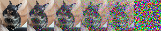
In contrast, latent representations tend to preserve a lot of signal structure. The figure below shows a few visualisations of Stable Diffusion latents for images (taken from the EQ-VAE paper33). It is pretty easy to identify the animals just from visually inspecting the latents. They basically look like noisy, low-resolution images with distorted colours. This is why I like to think of image latents as merely “advanced pixels”, capturing a little bit of extra information that regular pixels wouldn’t, but mostly still behaving like pixels nonetheless.
It is safe to say that these latents are quite low-level. Whereas traditional VAEs would compress an entire image into a single feature vector, often resulting in a high-level representation that enables semantic manipulation34, modern latent representations used for generative modelling of images are actually much closer to the pixel level. They are much higher-capacity, inheriting the grid structure of the input (though at a lower resolution). Each latent vector in the grid may abstract away some low-level image features such as textures, but it does not capture the semantics of the image content. This is also why most autoencoders do not make use of any additional conditioning signals such as text captions, as those mainly constrain high-level structure (though exceptions exist35).
Controlling capacity
Two key design parameters control the capacity of a grid-structured latent space: the downsampling factor and the number of channels of the representation. If the latent representation is discrete, the codebook size is also important, as it imposes a hard limit on the number of bits information that the latents can contain. (Aside from these, regularisation strategies play an important role, but we will discuss their impact in the next section.)
As an example, an encoder might take a 256×256 pixel image as input, and produce a 32×32 grid of continuous latent vectors with 8 channels. This could be achieved using a stack of strided convolutions, or perhaps using a vision Transformer (ViT)36 with patch size 8. The downsampling factor reduces the dimensionality along both width and height, so there are 64 times fewer latent vectors than pixels – but each latent vector has 8 components, while each pixel has only 3 (RGB). In aggregate, the latent representation is a tensor with \(\frac{w_{in} \cdot h_{in} \cdot c_{in}}{w_{out} \cdot h_{out} \cdot c_{out}} = \frac{256 \cdot 256 \cdot 3}{32 \cdot 32 \cdot 8} = 24\) times fewer components (i.e. floating point numbers) than the tensor representing the original image. I like to refer to this number as the tensor size reduction factor (TSR), to avoid confusion with spatial or temporal downsampling factors.
If we were to increase the downsampling factor of the encoder by 2×, the latent grid size would then be 16×16, and we could increase the channel count by 4× to 32 channels, to maintain the same TSR. There are usually a few different configurations for a given TSR that perform roughly equally in terms of reconstruction quality, especially in the case of video, where we can separately control the temporal and spatial downsampling factors. If we change the TSR, however (by changing the downsampling factor without changing the channel count, or vice versa), this usually has a profound impact on both reconstruction quality and modelability.
From a purely mathematical perspective, this is surprising: if the latents are real-valued, the size of the grid and the number of channels shouldn’t matter, because the information capacity of a single number is already infinite (neatly demonstrated by Tupper’s self-referential formula). But of course, there are several practical limitations that restrict the amount of information a single component of the latent representation is able to carry:
- we use floating point representations of real numbers, which have finite precision;
- in many formulations, the encoder adds some amount of noise, which further limits effective precision;
- neural networks aren’t very good at learning highly nonlinear functions of their input.
The first one is obvious: if you represent a number with 32 bits (single precision), that is also the maximal number of bits of information it can possibly convey. Adding noise further reduces the number of usable bits, because some of the low-order digits will be overpowered by it.
The last limitation is actually the more restrictive one, but it is less well understood: isn’t the entire point of neural networks to learn nonlinear functions? That is true, but they are naturally biased towards learning relatively simple functions37. This is usually a feature, not a bug, because it increases the probability of learning a function that generalises to unseen data. But if we are trying to compress a lot of information into a few numbers, that will likely require a high degree of nonlinearity. There are some ways to assist neural networks with learning more nonlinear functions (such as Fourier features38), but in our setting, highly nonlinear mappings will actually negatively affect modelability: they obfuscate signal structure, so this is not a good solution. Representations with more components offer a better trade-off.
The same applies to discrete latent representations: the discretisation imposes a hard limit on the information content of the representation, but whether that capacity can be used efficiently depends chiefly on how expressive the encoder is, and how well the quantisation strategy works in practice (i.e. whether it achieves a high level of codebook utilisation by using the different codes as evenly as possible). I believe the most commonly used approach today is still the original VQ bottleneck from VQ-VAE12, but a recent improvement which provides better gradient estimates using a “rotation trick”39 seems promising in terms of codebook utilisation and end-to-end performance. Some alternatives without explicitly learnt codebooks have also gained traction recently: finite scalar quantisation (FSQ)40, lookup-free quantisation (LFQ)41 and binary spherical quantisation (BSQ)42.
To recap, choosing the right TSR is key: a larger latent representation will yield better reconstruction quality (higher rate, lower distortion), but may negatively affect modelability. With a larger representation, there are simply more bits of information to model, therefore requiring more capacity in the generative model. In practice, this trade-off is usually tuned empirically. This can be an expensive affair, because there aren’t really any reliable proxy metrics for modelability that are cheap to compute. Therefore, it requires repeatedly training large enough generative models to get meaningful results.
Hansen-Estruch et al.43 recently shared an extensive exploration of latent space capacity and the various factors that influence it (their key findings are clearly highlighted within the text). There is currently a trend toward increasing the spatial downsampling factor, and maintaining the TSR by also increasing the number of channels accordingly, in order to facilitate image and video generation at higher resolutions (e.g. 32× in LTX-Video44 and GAIA-245, up to 64× in DCAE46).
Curating and shaping the latent space
So far, we have talked about the capacity of latent representations, i.e. how many bits of information should go in them. It is just as important to control precisely which bits from the original input signals should be preserved in the latents, and how this information is presented. I will refer to the former as curating the latent space, and to the latter as shaping the latent space – the distinction is subtle, but important. Many regularisation strategies have been devised to shape, curate and control the capacity of latents. I will focus on the continuous case, but many of the same considerations apply to discrete latents as well.
VQGAN and KL-regularised latents
Rombach et al.26 suggested two regularisation strategies for continuous latent spaces:
- Follow the original VQGAN recipe, reinterpreting the quantisation step as part of the decoder, rather than the encoder, to get a continuous representation (VQ-reg);
- Remove the quantisation step from the VQGAN recipe altogether, and replace it with a KL penalty, as in regular VAEs (KL-reg).
The idea of making only minimal changes to VQGAN to produce continuous latents (for use with diffusion models) is clever: the setup worked well for autoregressive models, and the quantisation during training serves as a safeguard to ensure that the latents don’t end up encoding too much information. However, as we discussed previously, this probably isn’t really necessary in most cases, because encoder expressivity is usually the limiting factor.
KL regularisation, on the other hand, is a core part of the traditional VAE setup: it is one of the two terms constituting the evidence lower bound (ELBO), which bounds the likelihood from below and enables VAE training to tractably (but indirectly) maximise the likelihood of the data. It encourages the latents to follow the imposed prior distribution (usually Gaussian). Crucially however, the ELBO is only truly a lower bound on the likelihood if there is no scaling hyperparameter in front of this term. Yet almost invariably, the KL term used to regularise continuous latent spaces is scaled down significantly (usually by several orders of magnitude), all but severing the connection with the variational inference context in which it originally arose.
The reason is simple: an unscaled KL term has too strong an effect, imposing a stringent limit on latent capacity and thus severely degrading reconstruction quality. The pragmatic response to that is naturally to scale down its relative contribution to the training loss. (Aside: in settings where one cares less about reconstruction quality, and more about semantic interpretability and disentanglement of the learnt representation, increasing the scale of the KL term can also be fruitful, as in beta-VAE34.)
We are veering firmly into opinion territory here, but I feel there is currently quite a bit of magical thinking around the effect of the KL term. It is often suggested that this term encourages the latents to follow a Gaussian distribution, but with the scale factors that are typically used, this effect is way too weak to be meaningful. Even for “proper” VAEs, the aggregate posterior is rarely actually Gaussian47 48.
All of this renders the “V” in “VAE” basically meaningless, in my opinion – its relevance is largely historical. We may as well drop it and talk about KL-regularised autoencoders instead, which more accurately reflects modern practice. The most important effect of the KL term in this setting is to supress outliers and constrain the scale of the latents to some extent. In other words: while the KL term is often presented as constraining capacity, the way it is used in practice mainly constrains the shape of the latents (but even that effect is relatively modest).
Tweaking reconstruction losses
The usual trio of reconstruction losses (regression, perceptual and adversarial) clearly plays an important role in maximising the quality of decoded signals, but it is also worth studying how these losses impact the latents, specifically in terms of curation (i.e. which information they learn to encode). As discussed in section 3, a good latent space in the visual domain makes abstraction of texture to some degree. How do these losses help achieve that?
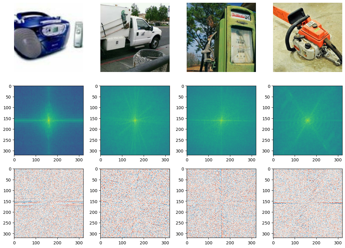
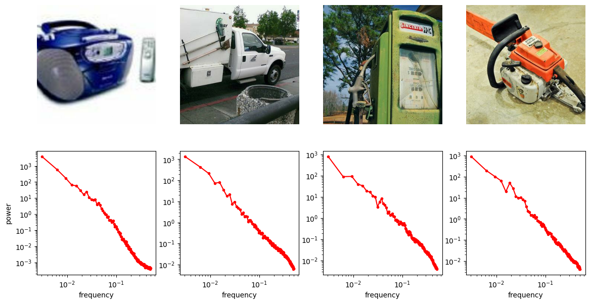
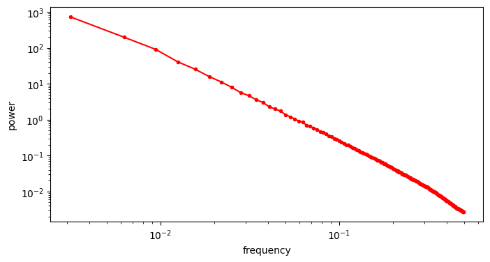
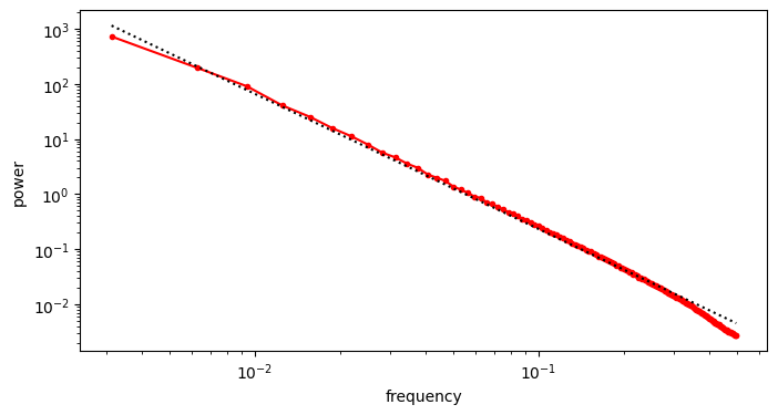
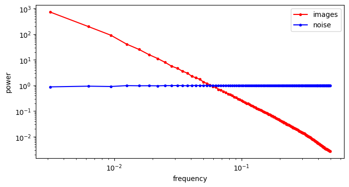
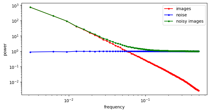
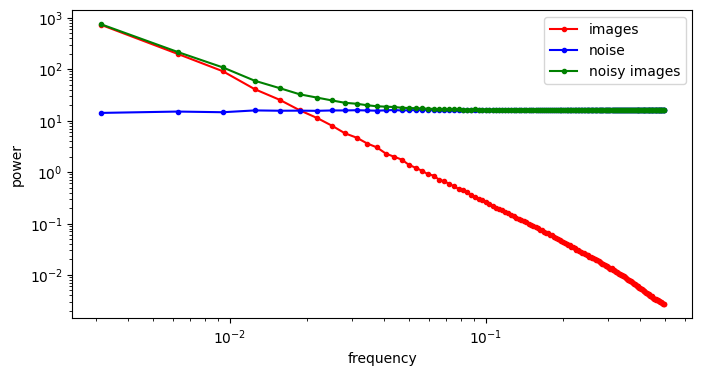
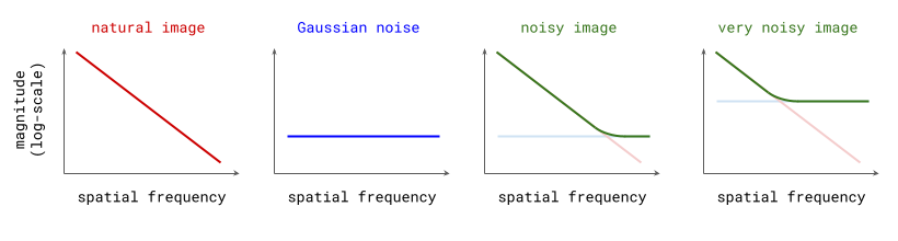
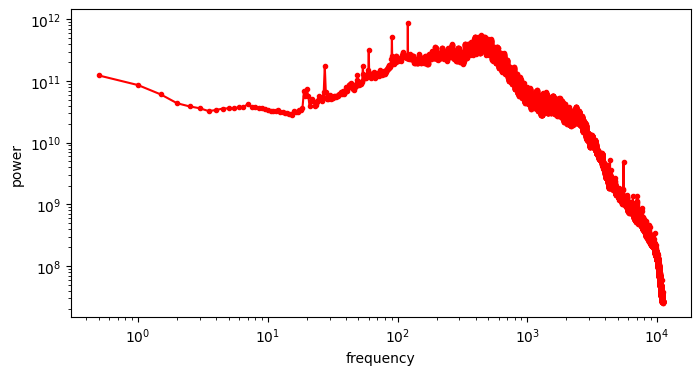
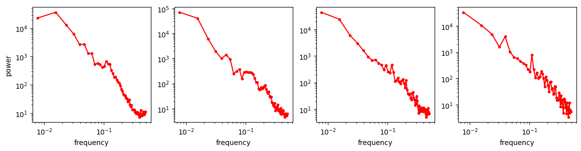
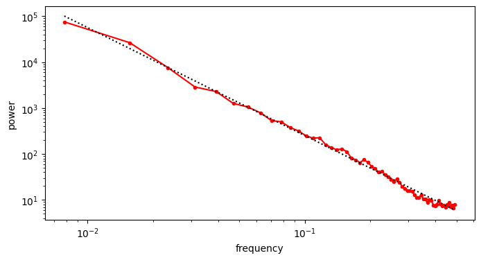
A useful thought experiment is to consider what happens when we drop the perceptual and adversarial losses, retaining only the regression loss, as in traditional VAEs. This will tend to result in blurry reconstructions. Regression losses do not favour any particular kind of signal content by design, so in the case of images, they will focus on low-frequency content, simply because there is more of it. In natural images, the power of different spatial frequencies tends to be proportional to their inverse square – the higher the frequency, the less power (see my previous blog post for an illustrated analysis of this phenomenon). Since high frequencies constitute only a tiny fraction of the total signal power, the regression loss more strongly rewards accurate prediction of low frequencies than high ones. The relative perceptual importance of these high frequencies is much larger than the fraction of total signal power they represent, and blurry looking reconstructions are the well-known result.
Since texture is primarily composed of precisely these high frequencies which the regression loss largely ignores, we end up with a latent space that doesn’t make abstraction of texture, but rather erases textural information altogether. From a perceptual standpoint, that is a particularly undesirable form of latent space curation. This demonstrates the importance of the other two reconstruction loss terms, which ensure that the latents can encode some textural information.
If the regression loss has these undesirable properties, which require other loss terms to mitigate, perhaps we could drop it altogether? It turns out that’s not a great idea either, because the perceptual and adversarial losses are much harder to optimise and tend to have pathological local minima (they are usually based on pre-trained neural networks, after all). The regression loss acts as a sort of regulariser, continually providing guardrails against ending up in the bad parts of parameter space as training progresses.
Many strategies using different flavours of reconstruction losses have been suggested, and I won’t cover this space exhaustively, but here are a few examples from the literature, to give you an idea of the variety:
- The aforementioned DCAE46 does not deviate too far from the original VQGAN recipe, only replacing the L2 regression loss (MSE) with L1 (MAE). It keeps the LPIPS perceptual loss and the PatchGAN49 discriminator. It does however use multiple stages of training, with the adversarial loss only enabled in the last stage.
- ViT-VQGAN50 combines two regression losses, the L2 loss and the logit-Laplace loss51, and uses the StyleGAN52 discriminator as well as the LPIPS perceptual loss.
- LTX-Video44 introduces a video-aware loss based on the discrete wavelet transform (DWT), and uses a modified strategy for the adversarial loss which they call reconstruction-GAN.
As with many classic dishes, every chef still has their own recipe!
Representation learning vs. reconstruction
The design choices we have discussed so far usually impact not just reconstruction quality, but also the kind of latent space that is learnt. The reconstruction losses in particular do double duty: they ensure high-quality decoder output, and play an important role in curating the latent space as well. This raises the question whether it is actually desirable to kill two birds with one stone, as we have been doing. I would argue that the answer is no.
Learning a good compact representation for generative modelling on the one hand, and learning to decode that representation back to the input space on the other hand, are two separate tasks. Modern autoencoders are expected to learn to do both at once. The fact that this works reasonably well in practice is certainly a welcome convenience: training an autoencoder is already stage one of a two-stage training process, so ideally we wouldn’t want to complicate it any further (although having multiple autoencoder training stages is not unheard of46 53). But this setup also needlessly conflates the two tasks, and some choices that are optimal for one task might not be for the other.
My colleagues and I actually made this point in a latent generative modelling paper54, all the way back in 2019 (I recently tweeted about it as well). When the decoder is autoregressive, conflating the two tasks is particularly problematic, so we suggested using a separate non-autoregressive auxiliary decoder to provide the learning signal for the encoder. The main decoder is prevented from influencing the latent representation at all, by not backpropagating its gradients through to the encoder. It is therefore fully focused on maximising reconstruction quality, while the auxiliary decoder takes care of shaping and curating the latent space. All parts of the autoencoder can still be trained jointly, so the additional complexity is limited. The auxiliary decoder does of course increase the cost of training, but it can be discarded afterwards.
Although the idea of using autoregressive decoders in pixel space, as we did for that paper, has not aged well at all (to put it mildly), I believe using auxiliary decoders to separate the representation learning and reconstruction tasks is still a very relevant idea today. An auxiliary decoder that optimises a different loss, or that has a different architecture (or both), could provide a better learning signal for representation learning and result in better generative modelling performance.
Zhu et al.55 recently came to the same conclusion (see section 2.1 of their paper), and constructed a discrete latent representation using K-means on DINOv256 features, combined with a separately trained decoder. Reusing representations learnt with self-supervised learning for generative modelling has historically been more common for audio models57 58 59 60 – perhaps because audio practitioners are already accustomed to the idea of training vocoders that turn predetermined intermediate representations (e.g. mel-spectrograms) back into audio waveforms.
Regularising for modelability
Shaping, curating and constraining the capacity of latents can all affect their modelability:
- Capacity constraints determine how much information is in the latents. The higher the capacity, the more powerful the generative model will have to be to adequately capture all of the information they contain.
- Shaping can be important to enable efficient modelling. The same information can be represented in many different ways, and some are easier to model than others. Scaling and standardisation are important to get right (especially for diffusion models), but higher-order statistics and correlation structure also matter.
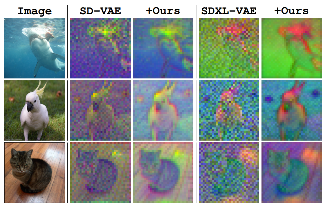
- Curation influences modelability, because some kinds of information are much easier to model than others. If the latents encode information about unpredictable noise in the input signal, that will make them less predictable as well. Here’s an interesting tweet that demonstrates how this affects the Stable Diffusion XL VAE61:
The sdxl-VAE models a substantial amount of noise. Things we can't even see. It meticulously encodes the noise, uses precious bottleneck capacity to store it, then faithfully reconstructs it in the decoder.
— Rudy Gilman (@rgilman33) April 14, 2025
I grabbed what I thought was a simple black vector circle on a white… pic.twitter.com/eK7ZtLJ6lc
Here, I want to make the connection to the idea of \(\mathcal{V}\)-information, proposed by Xu et al.62, which extends the concept of mutual information to account for computational constraints (h/t @jxmnop on Twitter for bringing this work to my attention). In other words, the usability of information varies depending on how computationally challenging it is for an observer to discern, and we can try to quantify this. If a piece of information requires a powerful neural net to extract, the \(\mathcal{V}\)-information in the input is lower than in the case where a simple linear probe suffices – even when the absolute information content measured in bits is identical. Clearly, maximising the \(\mathcal{V}\)-information of the latent representation is desirable, in order to minimise the computational requirements for the generative model to be able to make sense of it. The rate-distortion-usefulness trade-off described by Tschannen et al., which I mentioned before31, supports the same conclusion.
As discussed earlier, the KL penalty probably doesn’t do quite as much to Gaussianise or otherwise smoothen the latent space as many seem to believe. So what can we do instead to make the latents easier to model?
-
Use generative priors: co-train a (lightweight) latent generative model with the autoencoder, and make the latents easy to model by backpropagating the generative loss into the encoder, as in LARP63 or CRT64. This requires careful tuning of loss weights, because the generative loss and the reconstruction losses are at odds with each other: latents are easiest to model when they encode no information at all!
-
Supervise with pre-trained representations: encourage the latents to be predictive of existing high-quality representations (e.g. DINOv256 features), as in VA-VAE65, MAETok66 or GigaTok67.
-
Encourage equivariance: make it so that certain transformations of the input (e.g. rescaling, rotations) produce corresponding latent representations that are transformed similarly, as in AuraEquiVAE, EQ-VAE33 and AF-VAE68. The figure from the EQ-VAE paper that I used in section 4 shows the profound impact that this constraint can have on the spatial smoothness of the latent space. Skorokhodov et al.69 came to the same conclusion based on spectral analysis of latent spaces: equivariance regularisation makes the latent spectrum more similar to that of the pixel space inputs, which improves modelability.
This was just a small sample of possible regularisation strategies, all of which attempt to increase the \(\mathcal{V}\)-information of the latents in one way or another. This list is very far from exhaustive, both in terms of the strategies themselves and the works cited, so I encourage you to share any other relevant work you’ve come across in the comments!
Diffusion all the way down
A specific class of autoencoders for learning latent representations deserves a closer look: those with diffusion decoders. While a more typical decoder architecture features a feedforward network that directly outputs pixel values in one forward pass, and is trained adversarially, an alternative that’s gaining popularity is to use diffusion for the task of latent decoding (as well as for modelling the distribution of the latents). This impacts reconstruction quality, but it also affects what kind of representation is learnt.
SWYCC70, \(\epsilon\)-VAE71 and DiTo72 are some recent works that explore this approach. They motivate this in a few different ways:
- latents learnt with diffusion decoders provide a more principled, theoretically grounded way of doing hierarchical generative modelling;
- they can be trained with just the MSE loss, which simplifies things and improves robustness (adversarial losses are pretty finicky to tune, after all);
- applying the principle of iterative refinement to decoding improves output quality.
I can’t really argue with any of these points, but I do want to point out one significant weakness of diffusion decoders: their computational cost, and the effect this has on decoder latency. I believe one of the key reasons that most commercially deployed diffusion models today are latent models, is that compact latent representations help us avoid iterative refinement in input space, which is slow and costly. Performing the iterative sampling procedure in latent space, and then going back to input space with a single forward pass at the end, is significantly faster.
With that in mind, reintroducing input-space iterative refinement for the decoding task looks to me like it largely defeats the point of the two-stage approach. If we are going to be paying that cost, we might as well opt for something like simple diffusion73 74 to scale up single-stage generative models instead.
Not so fast, you might say – can’t we use one of the many diffusion distillation methods to bring down the number of steps required? In a setting such as this one, with a very rich conditioning signal (i.e. the latent representation), these methods have indeed proven effective even down to the single-step sampling regime: the stronger the conditioning, the fewer steps are needed for high quality distillation results.
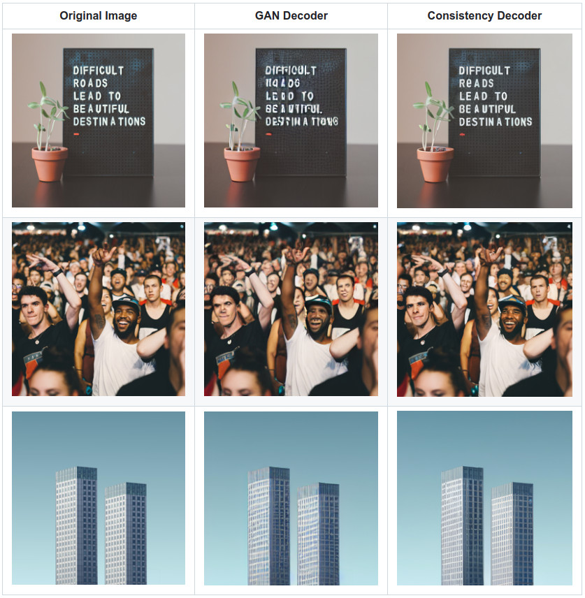
DALL-E 3’s consistency decoder75 is a great practical example of this: they reused the Stable Diffusion26 latent space and trained a new diffusion-based decoder, which was then distilled down to just two sampling steps using consistency distillation76. While it is still more costly than the original adversarial decoder in terms of latency, the visual fidelity of the outputs is significantly improved.
Music2Latent77 is another example of this approach, operating on spectrogram representations of music audio. Their autoencoder with a consistency decoder is trained end-to-end (unlike DALL-E 3’s, which reuses a pre-trained encoder), and is able to produce high-fidelity outputs in a single step. This means decoding once again requires only a single forward pass, as it does for adversarial decoders.
FlowMo53 is an autoencoder with a diffusion decoder that uses a post-training stage to encourage mode-seeking behaviour. As mentioned before, for the task of decoding latent representations, dropping modes and focusing on realism over diversity is actually desirable, because it requires less model capacity and does not negatively impact perceptual quality. Adversarial losses tend to result in mode dropping, but diffusion-based losses do not. This two-stage training strategy enables the diffusion decoder to mimic this behaviour – although a significant number of sampling steps are still required, so the computational cost is considerably higher than for a typical adversarial decoder.
Some earlier works on diffusion autoencoders, such as Diff-AE78 and DiffuseVAE79, are more focused on learning high-level semantic representations in the vein of old-school VAEs, without topological structure, and with a focus on controllability and disentanglement. DisCo-Diff80 sits somewhere in between, augmenting a diffusion model with a sequence of discrete latents, which can be modelled by an autoregressive prior.
Removing the need for adversarial training would certainly simplify things, so diffusion autoencoders are an interesting (and recently, quite popular) field of study in that regard. Still, it seems challenging to compete with adversarial decoders when it comes to latency, so I don’t think we are quite ready to abandon them. I very much look forward to an updated recipe that doesn’t require adversarial training, yet matches the current crop of adversarial decoders in terms of both visual quality and latency!
The tyranny of the grid

Digital representations of perceptual modalities are usually grid-structured, because they arise as uniformly sampled (and quantised) versions of the underlying physical signals. Images give rise to 2D grids of pixels, videos to 3D grids, and audio signals to 1D grids (i.e. sequences). The uniform sampling implies that there is a fixed quantum (i.e. distance or amount of time) between adjacent grid positions.
Perceptual signals also tend to be approximately stationary in time and space in a statistical sense. Combined with uniform sampling, this results in a rich topological structure, which we gratefully take advantage of when designing neural network architectures to process them: we use extensive weight sharing to benefit from invariance and equivariance properties, implemented through convolutions, recurrence and attention mechanisms.
Without a doubt, our ability to exploit this structure is one of the key reasons why we have been able to build machine learning models that are as powerful as they are. A corollary of this is that preserving this structure when designing latent spaces is a great idea. Our most powerful neural network designs architecturally depend on it, because they were originally built to process these digital signals directly. They will be better at processing latent representations instead, if those representations have the same kind of structure.
It also offers significant benefits for the autoencoders which learn to produce the latents: because of the stationarity, and because they only need to learn about local signal structure, they can be trained on smaller crops or segments of input signals. If we impose the right architectural constraints (limiting the receptive field of each position in the encoder and the decoder), they will generalise out of the box to larger grids than they were trained on. This has the potential to greatly reduce the training cost for the first stage.
It’s not all sunshine and rainbows though: we have discussed how perceptual signals are highly redundant, and unfortunately, this redundancy is unevenly distributed. Some parts of the signal might contain lots of detail that is perceptually salient, where others are almost devoid of information. In the image of a dog in a field that we used previously, consider a 100×100 pixel patch centered on the dog’s head, and then compare that to a 100×100 pixel patch in the top right corner of the image, which contains only the blue sky.
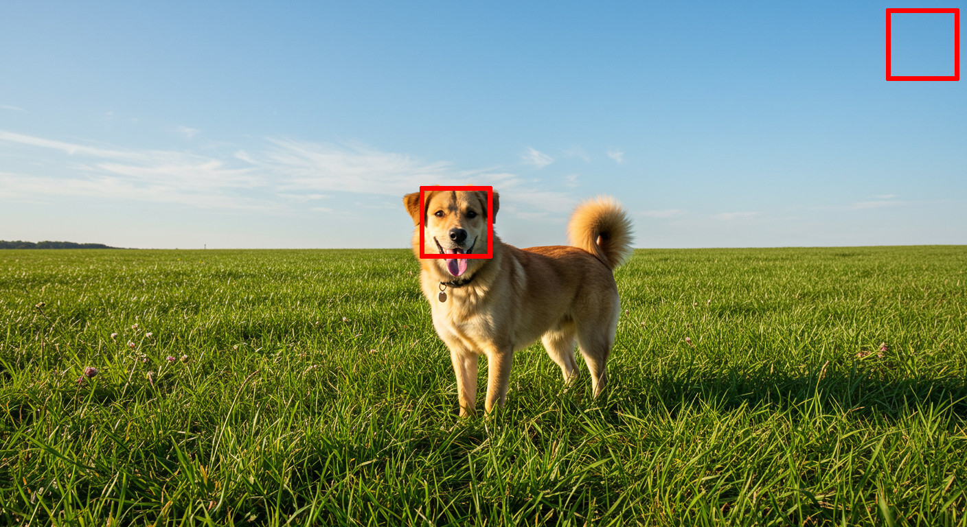
If we construct a latent representation which inherits the 2D grid structure of the input, and use it to encode this image, we will necessarily use the exact same amount of capacity to encode both of these patches. If we make the representation rich enough to capture all the relevant perceptual detail for the dog’s head, we will waste a lot of capacity to encode a similar-sized patch of sky. In other words, preserving the grid structure comes at a significant cost to the efficiency of the latent representation.
This is what I call the tyranny of the grid: our ability to process grid-structured data with neural networks is highly developed, and deviating from this structure adds complexity and makes the modelling task considerably harder and less hardware-friendly, so we generally don’t do this. But in terms of encoding efficiency, this is actually quite wasteful, because of the non-uniform distribution of perceptually salient information in audiovisual signals.
The Transformer architecture is actually relatively well-positioned to bolster a rebellion against this tyranny: while we often think of it as a sequence model, it is actually designed to process set-valued data, and any additional topological structure that relates elements of a set to each other is expressed through positional encoding. This makes deviating from a regular grid structure more practical than it is for convolutional or recurrent architectures. (Several years ago, my colleagues and I explored this idea for speech generation using variable-rate discrete representations81.)
Relaxing the topology of the latent space in the context of two-stage generative modelling appears to be gaining some traction lately:
- TiTok82 and FlowMo53 learn sequence-structured latents from images, reducing the grid dimensionality from 2D to 1D. The development of large language models has given us extremely powerful sequence models, so this is a reasonable kind of structure to aim for.
- One-D-Piece83, FlexTok84 and Semanticist85 do the same, but use a nested dropout mechanism86 to induce a coarse-to-fine structure in the latent sequence. This in turn enables the sequence length to be adapted to the complexity of each individual input image, and to the level of detail required in the reconstruction. A few other mechanisms for adaptive 1D tokenisation have been proposed, e.g. ElasticTok87 and ALIT88. CAT89 also explores this kind of adaptivity, but still maintains a 2D grid structure and only adapts its resolution.
- TokenSet90 goes a step further and uses an autoencoder that produces “bags of tokens”, abandoning the grid completely.
Aside from CAT, all of these have in common that they learn latent spaces that are considerably more semantically high-level than the ones we have mostly been talking about so far. In terms of abstraction level, they probably sit somewhere in the middle between “advanced pixels” and the vector-valued latents of old-school VAEs. In fact, FlexTok and Semanticist’s 1D sequence encoders expect low-level latents from an existing 2D grid-structured encoder as input, literally building an additional abstraction level on top of a pre-existing low-level latent space. TiTok and One-D-Piece also make use of an existing 2D grid-structured latent space as part of a multi-stage training approach. A related idea is to reuse the language domain as a high-level latent representation for images91.
In the discrete setting, some work has investigated whether commonly occurring patterns of tokens in a grid can be combined into larger sub-units, using ideas from language tokenisation: DiscreTalk92 is an early example in the speech domain, using SentencePiece93 on top of VQ tokens. Zhang et al.’s BPE Image Tokenizer94 is a more recent incarnation of this idea, using an enhanced byte-pair encoding95 algorithm on VQGAN tokens.
Latents for other modalities
We have chiefly focused on the visual domain so far, only briefly mentioning audio in some places. This is because learning latents for images is something we have gotten pretty good at, and image generation with the two-stage approach has been extensively studied (and productionised!) in recent years. We have a well-developed body of research on perceptual losses, and a host of discriminator architectures that enable adversarial training to focus on perceptually relevant image content.
With video, we remain in the visual domain, but a temporal dimension is introduced, which presents some challenges. One could simply reuse image latents and extract them frame-by-frame to get a latent video representation, but this would likely lead to temporal artifacts (like flickering). More importantly, it does not allow for taking advantage of temporal redundancy. I believe our tools for spatiotemporal latent representation learning are considerably less well developed, and how to account for the human perception of motion to improve efficiency is less well understood for now. This is in spite of the fact that video compression algorithms all make use of motion estimation to improve efficiency.
The same goes for audio: while there has been significant adoption of the two-stage recipe96 97 98, there seems to be considerably less of a broad consensus on the necessary modifications to make it work for this modality. As mentioned before, for audio it is also much more common to reuse representations learnt with self-supervised learning.
What about language? This is not a perceptual modality, but maybe the two-stage approach could improve the efficiency of large language models as well? This is not straightforward, as it turns out. Language is inherently much less compressible than perceptual signals: it developed as a means of efficient communication, so there is considerably less redundancy. Which is not to say there isn’t any: Shannon famously estimated English to be 50% redundant99. But recall that images, audio and video can be compressed by several orders of magnitude with relatively minimal perceptual distortion, which is not possible with language without losing nuance or important semantic information.
Tokenisers used for language models tend to be lossless (e.g. BPE95, SentencePiece93), so the resulting tokens aren’t usually viewed as “latents” (Byte Latent Transformer100 does use this framing for its dynamic tokenisation strategy, however). The relative lack of redundancy in language has not stopped people from trying to learn lossy higher-level representations, though! The techniques used for perceptual signals may not carry over, but several other methods to learn representations at the sentence or paragraph level have been explored101 102 103.
Will end-to-end win in the end?

When deep learning rose to prominence, the dominant narrative was that we would replace handcrafted features with end-to-end learning wherever possible. Jointly learning all processing stages would allow these stages to co-adapt and cooperate to maximise performance, while also simplifying things from an engineering perspective. This is more or less what ended up happening in computer vision and speech processing. In that light, it is rather ironic that the dominant generative modelling paradigm for perceptual signals today is a two-stage approach. Both stages tend to be learnt, but it’s not exactly end-to-end!
Text-to-image, text-to-video and text-to-audio models deployed in products today are, for the most part, using intermediate latent representations. It is worth pondering whether this is a temporary status quo, or likely to continue to be the case. Two-stage training does introduce a significant amount of complexity after all, and apart from being more elegant, end-to-end learning would help ensure that all parts of a system are perfectly in tune with a single, overarching objective.
As discussed, iterative refinement in the input space is slow and costly, and I think this is likely to remain the case for a while longer – especially as we continue to ramp up the quality, resolution and/or length of the generated signals. The benefits of latents for training efficiency and sampling latency are not something we are likely to be happy to give up on, and there are currently no viable alternatives that have been demonstrated to work at scale. This is somewhat of a contentious point, because some researchers seem to believe the time has come to move towards an end-to-end approach. Personally, I think it’s too early.
So, when will we be ready to move back to single-stage generative models? Methods like simple diffusion73 74, Ambient Space Flow Transformers104 and PixelFlow105 have shown that this already works pretty well, even at relatively high resolutions – it just isn’t very cost-effective yet. But hardware keeps getting better and faster at an incredible rate, so I suspect we will eventually reach a point where the relative inefficiency of input-space models starts to be economically preferable over the increased engineering complexity of latent-space models. When exactly this will happen depends on the modality, the rate of hardware improvements and research progress, so I will stop short of making a concrete prediction.
It used to be the case that we needed latents to ensure that generative models would focus on learning about perceptually relevant signal content, while ignoring entropy that is not visually salient. Recall that the likelihood loss in input space is particularly bad at this, and switching to measuring likelihood in latent space dramatically improved results obtained with likelihood-based models12. Arguably, this is no longer the case, because we have figured out how to perceptually re-weight the likelihood loss function for both autoregressive and diffusion models106 107, removing an important obstacle to scaling. But in spite of that, the computational efficiency benefits of latent-space models remain as relevant as ever.
A third alternative, which I’ve only briefly mentioned so far, is the resolution cascade approach. This requires no representation learning, but still splits up the generative modelling problem into multiple stages. Some early commercial models used this approach, but it seems to have fallen out of favour. I believe this is because the division of labour between the different stages is suboptimal – upsampling models have to do too much of the work, and this makes them more prone to error accumulation across stages.
Closing thoughts
To wrap up, here are some key takeaways:
- Latents for generative modelling are usually quite unlike VAE latents from way back when: it makes more sense to think of them as advanced pixels than as high-level semantic representations.
- Having two stages enables us to have different loss functions for each, and significantly improves computational efficiency by avoiding iterative sampling in the input space.
- Latents add complexity, but the computational efficiency benefits are large enough for us to tolerate this complexity – at least for now.
- Three main aspects to consider when designing latent spaces are capacity (how many bits of information are encoded in the latents), curation (which bits from the input signals are retained) and shape (how this information is presented).
- Preserving structure (i.e. topology, statistics) in the latent space is important to make it easy to model, even if this is sometimes worse from an efficiency perspective.
- The V in VAE is vestigial: the autoencoders used in two-stage latent generative models are really KL-regularised AEs, and usually barely regularised at that.
- The combination of a regression loss, a perceptual loss and an adversarial loss is surprisingly entrenched. Almost all modern implementations of autoencoders for latent representation learning are variations on this theme.
- Representation learning and reconstruction are two separate tasks, and while it is convenient to do both at once, this might not be optimal.
Several years ago, I wrote on this blog that representation learning has an important role to play in generative modelling. Though it wasn’t exactly prophetic at the time (VQ-VAE had already existed for three years), the focus in the representation learning community back then was firmly on high-level semantic representations that are useful for discriminative tasks. It was a lot more common to hear about generative modelling in service of representation learning, than vice versa. How the tables have turned! The arrival of VQGAN16 a few months later was probably what cemented the path we now find ourselves on, and made two-stage generative modelling go mainstream.
Thank you for reading what ended up being my longest blog post yet! I’m keen to hear your thoughts here in the comments, on Twitter (yes, that’s what I’m calling it), or on BlueSky.
If you would like to cite this post in an academic context, you can use this BibTeX snippet:
@misc{dieleman2025latents,
  author = {Dieleman, Sander},
  title = {Generative modelling in latent space},
  url = {https://sander.ai/2025/04/15/latents.html},
  year = {2025}
}
Acknowledgements
Thanks to my colleagues at Google DeepMind for various discussions, which continue to shape my thoughts on this topic! Thanks also to Stefan Baumann, Rami Seid, Charles Foster, Ethan Smith, Simo Ryu, Theodoros Kouzelis and Jack Gallagher.
References
-
Zhang, Isola, Efros, Shechtman, Wang, “The Unreasonable Effectiveness of Deep Features as a Perceptual Metric”, Computer Vision and Pattern Recognition, 2018. ↩
-
Goodfellow, Pouget-Abadie, Mirza, Xu, Warde-Farley, Ozair, Courville and Bengio, “Generative Adversarial Nets”, Advances in neural information processing systems 27 (NeurIPS), 2014. ↩ ↩2
-
Van den Oord, Kalchbrenner and Kavukcuoglu, “Pixel recurrent neural networks”, International Conference on Machine Learning, 2016. ↩
-
Van den Oord, Kalchbrenner, Espeholt, Vinyals and Graves, “Conditional image generation with pixelcnn decoders”, Advances in neural information processing systems 29 (NeurIPS), 2016. ↩
-
Van den Oord, Dieleman, Zen, Simonyan, Vinyals, Graves, Kalchbrenner, Senior and Kavukcuoglu, “WaveNet: A Generative Model for Raw Audio”, arXiv, 2016. ↩
-
Mehri, Kumar, Gulrajani, Kumar, Jain, Sotelo, Courville and Bengio, “SampleRNN: An Unconditional End-to-End Neural Audio Generation Model”, International Conference on Learning Representations, 2017. ↩
-
Sohl-Dickstein, Weiss, Maheswaranathan and Ganguli, “Deep Unsupervised Learning using Nonequilibrium Thermodynamics”, International Conference on Machine Learning, 2015. ↩
-
Song and Ermon, “Generative Modeling by Estimating Gradients of the Data Distribution”, Neural Information Processing Systems, 2019. ↩
-
Ho, Jain and Abbeel, “Denoising Diffusion Probabilistic Models”, Neural Information Processing Systems, 2020. ↩
-
Chen, Zhang, Zen, Weiss, Norouzi, Chan, “WaveGrad: Estimating Gradients for Waveform Generation”, International Conference on Learning Representations, 2021. ↩
-
Kong, Ping, Huang, Zhao, Catanzaro, “DiffWave: A Versatile Diffusion Model for Audio Synthesis”, International Conference on Learning Representations, 2021. ↩
-
van den Oord, Vinyals and Kavukcuoglu, “Neural Discrete Representation Learning”, Neural Information Processing Systems, 2017. ↩ ↩2 ↩3
-
Kingma and Welling, “Auto-Encoding Variational Bayes”, International Conference on Learning Representations, 2014. ↩
-
Rezende, Mohamed and Wierstra, “Stochastic Backpropagation and Approximate Inference in Deep Generative Models”, International Conference on Machine Learning, 2014. ↩
-
Razavi, van den Oord and Vinyals, “Generating Diverse High-Fidelity Images with VQ-VAE-2”, Neural Information Processing Systems, 2019. ↩
-
Esser, Rombach and Ommer, “Taming Transformers for High-Resolution Image Synthesis”, Computer Vision and Pattern Recognition, 2021. ↩ ↩2 ↩3
-
Yu, Xu, Koh, Luong, Baid, Wang, Vasudevan, Ku, Yang, Ayan, Hutchinson, Han, Parekh, Li, Zhang, Baldridge, Wu, “Scaling Autoregressive Models for Content-Rich Text-to-Image Generation”, Transactions on Machine Learning, Research, 2022. ↩
-
Vaswani, Shazeer, Parmar, Uszkoreit, Jones, Gomez, Kaiser and Polosukhin, “Attention is All you Need”, Advances in neural information processing systems 30 (NeurIPS), 2017. ↩
-
Kingma, Ba, “Adam: A Method for Stochastic Optimization”, International Conference on Learning Representations, 2015. ↩
-
Tschannen, Eastwood, Mentzer, “GIVT: Generative Infinite-Vocabulary Transformers”, European Conference on Computer Vision, 2024. ↩
-
Li, Tian, Li, Deng, He, “Autoregressive Image Generation without Vector Quantization”, Neural Information Processing Systems, 2024. ↩
-
Mittal, Engel, Hawthorne, Simon, “Symbolic Music Generation with Diffusion Models”, International Society for Music Information Retrieval, 2021. ↩ ↩2
-
Vahdat, Kreis, Kautz, “Score-based Generative Modeling in Latent Space”, Neural Information Processing Systems, 2021. ↩ ↩2
-
Sinha, Song, Meng, Ermon, “D2C: Diffusion-Decoding Models for Few-Shot Conditional Generation”, Neural Information Processing Systems, 2021. ↩ ↩2
-
Wehenkel, Louppe, “Diffusion Priors In variational Autoencoders”, International Conference on Machine Learning workshop, 2021. ↩ ↩2
-
Rombach, Blattmann, Lorenz, Esser, Ommer, “High-Resolution Image Synthesis with Latent Diffusion Models”, Computer Vision and Pattern Recognition, 2022. ↩ ↩2 ↩3 ↩4
-
Ostrovski, Dabney and Munos, “Autoregressive Quantile Networks for Generative Modeling”, International Conference on Machine Learning, 2018. ↩
-
Nash, Menick, Dieleman, Battaglia, “Generating Images with Sparse Representations”, International Conference on Machine Learning, 2021. ↩
-
Nash, Carreira, Walker, Barr, Jaegle, Malinowski, Battaglia, “Transframer: Arbitrary Frame Prediction with Generative Models”, Transactions on Machine Learning Research, 2023. ↩
-
Han, Ghazvininejad, Koh, Tsvetkov, “JPEG-LM: LLMs as Image Generators with Canonical Codec Representations”, arXiv, 2024. ↩
-
Tschannen, Bachem, Lucic, “Recent Advances in Autoencoder-Based Representation Learning”, Neural Information Processing Systems workshop, 2018. ↩ ↩2
-
Blau, Michaeli, “Rethinking Lossy Compression: The Rate-Distortion-Perception Tradeoff”, International Conference on Machine Learning, 2019. ↩
-
Kouzelis, Kakogeorgiou, Gidaris, Komodakis, “EQ-VAE: Equivariance Regularized Latent Space for Improved Generative Image Modeling”, arXiv, 2025. ↩ ↩2
-
Higgins, Matthey, Pal, Burgess, Glorot, Botvinick, Mohamed, Lerchner, “β-VAE: Learning Basic Visual Concepts with a Constrained Variational Framework”, International Conference on Learning Representations, 2017. ↩ ↩2
-
Zha, Yu, Fathi, Ross, Schmid, Katabi, Gu, “Language-Guided Image Tokenization for Generation”, Computer Vision and Pattern Recognition, 2025. ↩
-
Dosovitskiy, Beyer, Kolesnikov, Weissenborn, Zhai, Unterhiner, Dehghani, Minderer, Heigold, Gelly, Uszkoreit, Houlsby, “[An Image is Worth 16x16 Words: Transformers for Image Recognition at Scale]”, International Conference on Learning Representations, 2021. ↩
-
Rahaman, Baratin, Arpit, Draxler, Lin, Hamprecht, Bengio, Courville, “On the Spectral Bias of Neural Networks”, International Conference on Machine Learning, 2019. ↩
-
Tancik, Srinivasan, Mildenhall, Fridovich-Keil, Raghavan, Singhal, Ramamoorthi, Barron, Ng, “Fourier Features Let Networks Learn High Frequency Functions in Low Dimensional Domains”, Neural Information Processing Systems, 2020. ↩
-
Fifty, Junkins, Duan, Iyengar, Liu, Amid, Thrun, Ré, “Restructuring Vector Quantization with the Rotation Trick”, International Conference on Learning Representations, 2025. ↩
-
Mentzer, Minnen, Agustsson, Tschannen, “Finite Scalar Quantization: VQ-VAE Made Simple”, International Conference on Learning Representations, 2024. ↩
-
Yu, Lezama, Gundavarapu, Versari, Sohn, Minnen, Cheng, Birodkar, Gupta, Gu, Hauptmann, Gong, Yang, Essa, Ross, Jiang, “Language Model Beats Diffusion – Tokenizer is Key to Visual Generation”, International Conference on Learning Representations, 2024. ↩
-
Zhao, Xiong, Krähenbühl, “Image and Video Tokenization with Binary Spherical Quantization”, arXiv, 2024. ↩
-
Hansen-Estruch, Yan, Chung, Zohar, Wang, Hou, Xu, Vishwanath, Vajda, Chen, “Learnings from Scaling Visual Tokenizers for Reconstruction and Generation”, arXiv, 2025. ↩
-
HaCohen, Chiprut, Brazowski, Shalem, Moshe, Richardson, Levin, Shiran, Zabari, Gordon, Panet, Weissbuch, Kulikov, Bitterman, Melumian, Bibi, “LTX-Video: Realtime Video Latent Diffusion”, arXiv, 2024. ↩ ↩2
-
Russell, Hu, Bertoni, Fedoseev, Shotton, Arani, Corrado, “GAIA-2: A Controllable Multi-View Generative World Model for Autonomous Driving”, arXiv, 2025. ↩
-
Chen, Cai, Chen, Xie, Yang, Tang, Li, Lu, Han, “Deep Compression Autoencoder for Efficient High-Resolution Diffusion Models”, International Conference on Learning Representations, 2025. ↩ ↩2 ↩3
-
Rosca, Lakshminarayanan, Mohamed, “Distribution Matching in Variational Inference”, arXiv 2018. ↩
-
Hoffman, Johnson, “ELBO surgery: yet another way to carve up the variational evidence lower bound”, Neural Information Processing Systems, 2016. ↩
-
Isola, Zhu, Zhou, Efros, “Image-to-Image Translation with Conditional Adversarial Networks”, Computer Vision and Pattern Recognition, 2017. ↩
-
Yu, Li, Koh, Zhang, Pang, Qin, Ku, Xu, Baldridge, Wu, “Vector-quantized Image Modeling with Improved VQGAN”, International Conference on Learning Representations, 2022. ↩
-
Ramesh, Pavlov, Goh, Gray, Voss, Radford, Chen, Sutskever, “Zero-Shot Text-to-Image Generation”, International Conference on Machine Learning, 2021. ↩
-
Karras, Laine, Aittala, Hellsten, Lehtinen, Aila, “Analyzing and Improving the Image Quality of StyleGAN”, Computer Vision and Pattern Recognition, 2020. ↩
-
Sargent, Hsu, Johnson, Li, Wu, “Flow to the Mode: Mode-Seeking Diffusion Autoencoders for State-of-the-Art Image Tokenization”, arXiv, 2025. ↩ ↩2 ↩3
-
De Fauw, Dieleman, Simonyan, “Hierarchical Autoregressive Image Models with Auxiliary Decoders”, arXiv, 2019. ↩
-
Zhu, Li, Zhang, Li, Xu, Bing, “Stabilize the Latent Space for Image Autoregressive Modeling: A Unified Perspective”, Neural Information Processing Systems, 2024. ↩
-
Oquab, Darcet, Moutakanni, Vo, Szafraniec, Khalidov, Fernandez, Haziza, Massa, El-Nouby, Assran, Ballas, Galuba, Howes, Huang, Li, Misra, Rabbat, Sharma, Synnaeve, Xu, Jegou, Mairal, Labatut, Joulin, Bojanowski, “DINOv2: Learning Robust Visual Features without Supervision”, Transactions on Machine Learning Research, 2024. ↩ ↩2
-
Hadjeres, Crestel, “Vector Quantized Contrastive Predictive Coding for Template-based Music Generation”, arXiv, 2020. ↩
-
Lakhotia, Kharitonov, Hsu, Adi, Polyak, Bolte, Nguyen, Copet, Baevski, Mohamed, Dupoux, “Generative Spoken Language Modeling from Raw Audio”, Transactions of the Association for Computational Linguistics, 2021. ↩
-
Borsos, Marinier, Vincent, Kharitonov, Pietquin, Sharifi, Roblek, Teboul, Grangier, Tagliasacchi, Zeghidour, “AudioLM: a Language Modeling Approach to Audio Generation”, Transactions on Audio, Speech and Language Processing, 2023. ↩
-
Mousavi, Duret, Zaiem, Della Libera, Ploujnikov, Subakan, Ravanelli, “How Should We Extract Discrete Audio Tokens from Self-Supervised Models?”, Interspeech, 2024. ↩
-
Podell, English, Lacey, Blattmann, Dockhorn, Müller, Penna, Rombach, “SDXL: Improving Latent Diffusion Models for High-Resolution Image Synthesis”, International Conference on Learning Representations, 2024. ↩
-
Xu, Zhao, Song, Stewart, Ermon, “A Theory of Usable Information Under Computational Constraints”, International Conference on Learning Representations, 2020. ↩
-
Wang, Suri, Ren, Chen, Shrivastava, “LARP: Tokenizing Videos with a Learned Autoregressive Generative Prior”, International Conference on Learning Representations, 2025. ↩
-
Ramanujan, Tirumala, Aghajanyan, Zettlemoyer, Farhadi, “When Worse is Better: Navigating the compression-generation tradeoff in visual tokenization”, arXiv, 2024. ↩
-
Yao, Yang, Wang, “Reconstruction vs. Generation: Taming Optimization Dilemma in Latent Diffusion Models”, Computer Vision and Pattern Recognition, 2025. ↩
-
Chen, Han, Chen, Li, Wang, Wang, Wang, Liu, Zou, Raj, “Masked Autoencoders Are Effective Tokenizers for Diffusion Models”, arXiv, 2025. ↩
-
Xiong, Liew, Huang, Feng, Liu, “GigaTok: Scaling Visual Tokenizers to 3 Billion Parameters for Autoregressive Image Generation”, arXiv, 2025. ↩
-
Zhou, Xiao, Yang, Pan, “Alias-Free Latent Diffusion Models: Improving Fractional Shift Equivariance of Diffusion Latent Space”, Computer Vision and Pattern Recognition, 2025. ↩
-
Skorokhodov, Girish, Hu, Menapace, Li, Abdal, Tulyakov, Siarohin, “Improving the Diffusability of Autoencoders”, arXiv, 2025. ↩
-
Birodkar, Barcik, Lyon, Ioffe, Minnen, Dillon, “Sample what you cant compress”, arXiv, 2024. ↩
-
Zhao, Woo, Zan, Li, Zhang, Gong, Adam, Jia, Liu, “Epsilon-VAE: Denoising as Visual Decoding”, arXiv, 2024. ↩
-
Chen, Girdhar, Wang, Rambhatla, Misra, “Diffusion Autoencoders are Scalable Image Tokenizers”, arXiv, 2025. ↩
-
Hoogeboom, Heek, Salimans, “Simple diffusion: End-to-end diffusion for high resolution images”, International Conference on Machine Learning, 2023. ↩ ↩2
-
Hoogeboom, Mensink, Heek, Lamerigts, Gao, Salimans, “Simpler Diffusion (SiD2): 1.5 FID on ImageNet512 with pixel-space diffusion”, Computer Vision and Pattern Recognition, 2025. ↩ ↩2
-
Betker, Goh, Jing, Brooks, Wang, Li, Ouyang, Zhuang, Lee, Guo, Manassra, Dhariwal, Chu, Jiao, Ramesh, “Improving Image Generation with Better Captions”, 2023. ↩
-
Song, Dhariwal, Chen, Sutskever, “Consistency Models”, International Conference on Machine Learning, 2023. ↩
-
Pasini, Lattner, Fazekas, “Music2Latent: Consistency Autoencoders for Latent Audio Compression”, International Society for Music Information Retrieval conference, 2024. ↩
-
Preechakul, Chatthee, Wizadwongsa, Suwajanakorn, “Diffusion Autoencoders: Toward a Meaningful and Decodable Representation”, Computer Vision and Pattern Recognition, 2022. ↩
-
Pandey, Mukherjee, Rai, Kumar, “DiffuseVAE: Efficient, Controllable and High-Fidelity Generation from Low-Dimensional Latents”, arXiv, 2022. ↩
-
Xu, Corso, Jaakkola, Vahdat, Kreis, “DisCo-Diff: Enhancing Continuous Diffusion Models with Discrete Latents”, International Conference on Machine Learning, 2024. ↩
-
Dieleman, Nash, Engel, Simonyan, “Variable-rate discrete representation learning”, arXiv, 2021. ↩
-
Yu, Weber, Deng, Shen, Cremers, Chen, “An Image is Worth 32 Tokens for Reconstruction and Generation”, Neural Information Processing Systems, 2024. ↩
-
Miwa, Sasaki, Arai, Takahashi, Yamaguchi, “One-D-Piece: Image Tokenizer Meets Quality-Controllable Compression”, arXiv, 2025. ↩
-
Bachmann, Allardice, Mizrahi, Fini, Kar, Amirloo, El-Nouby, Zamir, Dehghan, “FlexTok: Resampling Images into 1D Token Sequences of Flexible Length”, arXiv, 2025. ↩
-
Wen, Zhao, Elezi, Deng, Qi, ““Principal Components” Enable A New Language of Images”, arXiv, 2025. ↩
-
Rippel, Gelbart, Adams, “Learning Ordered Representations with Nested Dropout”, International Conference on Machine Learning, 2014. ↩
-
Yan, Mnih, Faust, Zaharia, Abbeel, Liu, “ElasticTok: Adaptive Tokenization for Image and Video”, International Conference on Learning Representations, 2025. ↩
-
Duggal, Isola, Torralba, Freeman, “Adaptive Length Image Tokenization via Recurrent Allocation”, International Conference on Learning Representations, 2025. ↩
-
Shen, Tirumala, Yasunaga, Misra, Zettlemoyer, Yu, Zhou, “CAT: Content-Adaptive Image Tokenization”, arXiv, 2025. ↩
-
Geng, Xu, Hu, Gu, “Tokenize Image as a Set”, arXiv, 2025. ↩
-
Wang, Zhou, Fathi, Darrell, Schmid, “Visual Lexicon: Rich Image Features in Language Space”, arXiv, 2024. ↩
-
Hayashi, Watanabe, “DiscreTalk: Text-to-Speech as a Machine Translation Problem”, Interspeech, 2020. ↩
-
Kudo, Richardson, “SentencePiece: A simple and language independent subword tokenizer and detokenizer for Neural Text Processing”, Empirical Methods in Natural Language Processing, 2018. ↩ ↩2
-
Zhang, Xie, Feng, Li, Xing, Zheng, Lu, “From Pixels to Tokens: Byte-Pair Encoding on Quantized Visual Modalities”, International Conference on Learning Representations, 2025. ↩
-
Gage, “A New Algorithm for Data Compression”, The C User Journal, 1994. ↩ ↩2
-
Zeghidour, Luebs, Omran, Skoglund, Tagliasacchi, “SoundStream: An End-to-End Neural Audio Codec”, Transactions on Audio, Speech and Language Processing, 2021. ↩
-
Défossez, Copet, Synnaeve, Adi, “High Fidelity Neural Audio Compression”, Transactions on Machine Learning Research, 2023. ↩
-
Kumar, Seetharaman, Luebs, Kumar, Kumar, “High-Fidelity Audio Compression with Improved RVQGAN”, Neural Information Processing Systems, 2023. ↩
-
Shannon, “A mathematical theory of communication”, The Bell System Technical Journal, 1948. ↩
-
Pagnoni, Pasunuru, Rodriguez, Nguyen, Muller, Li, Zhou, Yu, Weston, Zettlemoyer, Ghosh, Lewis, Holtzman, Iyer, “Byte Latent Transformer: Patches Scale Better Than Tokens”, arXiv, 2024. ↩
-
Wang, Durmus, Goodman, Hashimoto, “Language modeling via stochastic processes”, International Conference on Learning Representations, 2022. ↩
-
Zhang, Gu, Wu, Zhai, Susskind, Jaitly, “PLANNER: Generating Diversified Paragraph via Latent Language Diffusion Model”, Neural Information Processing Systems, 2023. ↩
-
Barrault, Duquenne, Elbayad, Kozhevnikov, Alastruey, Andrews, Coria, Couairon, Costa-jussà, Dale, Elsahar, Heffernan, Janeiro, Tran, Ropers, Sánchez, San Roman, Mourachko, Saleem, Schwenk, “Large Concept Models: Language Modeling in a Sentence Representation Space”, arXiv, 2024. ↩
-
Wang, Ranjan, Susskind, Bautista, “Coordinate In and Value Out: Training Flow Transformers in Ambient Space”, arXiv, 2024. ↩
-
Chen, Ge, Zhang, Sun, Luo, “PixelFlow: Pixel-Space Generative Models with Flow”, arXiv, 2025. ↩
-
Kingma, Gao, “Understanding Diffusion Objectives as the ELBO with Simple Data Augmentation”, Neural Information Processing Systems, 2024. ↩
-
Tschannen, Pinto, Kolesnikov, “JetFormer: An Autoregressive Generative Model of Raw Images and Text”, arXiv, 2024. ↩