The Galaxy Zoo challenge on Kaggle has just finished. The goal of the competition was to predict how Galaxy Zoo users (zooites) would classify images of galaxies from the Sloan Digital Sky Survey. I finished in 1st place and in this post I’m going to explain how my solution works.
Introduction
The problem
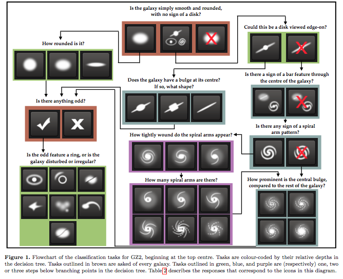
Galaxy Zoo is a crowdsourcing project, where users are asked to describe the morphology of galaxies based on images. They are asked questions such as “How rounded is the galaxy” and “Does it have a central bulge”, and the users’ answers determine which question will be asked next. The questions form a decision tree which is shown in the figure below, taken from Willett et al. 2013.

When many users have classified the same image, their answers can be aggregated into a set of probabilities for each answer. Often, not all users will agree on all of their answers, so it’s useful to quantify this uncertainty.
The goal of the Galaxy Zoo challenge is to predict these probabilities from the galaxy images that are shown to the users. In other words, build a model of how “the crowd” perceive and classify these images.
This means that we’re looking at a regression problem, not a classification problem: we don’t have to determine which classes the galaxies belong to, but rather the fraction of people who would classify them as such.
My solution: convnets
I suppose this won’t surprise anyone: my solution is based around convolutional neural networks (convnets). I believe they’re an excellent match for this problem: it’s image data, but it is different enough from typical image data (i.e. “natural” images such as those used in object recognition, scene parsing, etc.) for traditional features from computer vision to be suboptimal. Learning the features just seems to make sense.
Transfer learning by pre-training a deep neural network on another dataset (say, ImageNet), chopping off the top layer and then training a new classifier, a popular approach for the recently finished Dogs vs. Cats competition, is not really viable either. There were no requests to use external data in the competition forums (a requirement to be allowed to use it), so I guess nobody tried this approach.
During the contest, I frequently referred to Krizhevsky et al.’s seminal 2012 paper on ImageNet classification for guidance. Asking myself “What would Krizhevsky do?” usually resulted in improved performance.
Overfitting
As Geoffrey Hinton has been known to say, if you’re not overfitting, your network isn’t big enough. My main objective during the competition was avoiding overfitting. My models were significantly overfitting throughout the entire competition, and most of the progress I attained came from finding new ways to mitigate that problem.
I tackled this problem with three orthogonal approaches:
- data augmentation
- dropout and weight norm constraints
- modifying the network architecture to increase parameter sharing
The best model I found has about 42 million parameters. It overfits significantly, but it’s still the best despite that. There seems to be a lot of room for improvement there.
As is customary in Kaggle competitions, I also improved my score quite a bit by averaging the predictions of a number of different models. Please refer to the “Model averaging” section below for more details.
Software and hardware
I used Python, NumPy and Theano to implement my solution. I also used the Theano wrappers for the cuda-convnet convolution implementation that are part of pylearn2. They provided me with a speed boost of almost 3x over Theano’s own implementation. I wrote a guide on how to use them, because their documentation is limited.
I used scikit-image for preprocessing and augmentation. I also used sextractor and pysex to extract some parameters of the galaxies from the images.
The networks were trained on workstations with a hexacore CPU, 32GB RAM and two NVIDIA GeForce GTX 680 GPUs each.
Preprocessing and data augmentation
Cropping and downsampling
The data consisted of 424x424 colour JPEG images, along with 37 weighted probabilities that have to be predicted for each image (for details on the weighting scheme, please refer to this page).
For almost all of the images, the interesting part was in the center. The void of space around the galaxies was not very discriminative, so I cropped all images to 207x207. I then downsampled them 3x to 69x69, to keep the input size of the network manageable.
Exploiting spatial invariances
Images of galaxies are rotation invariant: there is no up or down in space. They are also scale invariant and translation invariant to a limited extent. All of these invariances could be exploited to do data augmentation: creating new training data by perturbing the existing data points.
Each training example was perturbed before presenting it to the network by randomly scaling it, rotating it, translating it and optionally flipping it. I used the following parameter ranges:
- rotation: random with angle between 0° and 360° (uniform)
- translation: random with shift between -4 and 4 pixels (relative to the original image size of 424x424) in the x and y direction (uniform)
- zoom: random with scale factor between 1/1.3 and 1.3 (log-uniform)
- flip: yes or no (bernoulli)
Because both the initial downsampling to 69x69 and the random perturbation are affine transforms, they could be combined into one affine transformation step (I used scikit-image for this). This sped up things significantly and reduced information loss.
Colour perturbation
After this, the colour of the images was changed as described in Krizhevsky et al. 2012, with two differences: the first component had a much larger eigenvalue than the other two, so only this one was used, and the standard deviation for the scale factor alpha was set to 0.5.
“Realtime” augmentation
Combining downsampling and perturbation into a single affine transform made it possible to do data augmentation in realtime, i.e. during training. This significantly reduced overfitting because the network would never see the exact same image twice. While the network was being trained on a chunk of data on the GPU, the next chunk would be generated on the CPU in multiple processes, to ensure that all the available cores were used.
Centering and rescaling
I experimented with centering and rescaling the galaxy images based on parameters extracted with sextractor. Although this didn’t improve performance, including a few models that used it in the final ensemble helped to increase variance (see “Model averaging” for more information).
I extracted the center of the galaxies, as well as the Petrosian radius. A number of different radii can be extracted, but the Petrosian radius seemed to give the best size estimate. I then centered each image by shifting the estimated center pixel to (212, 212), and rescaled it so that its Petrosian radius would be equal to 160 pixels. The scale factor was limited to the range (1/1.5, 1.5), because there were some outliers.
This rescaling and centering could also be collapsed into the affine transform doing downsampling and perturbation, so it did not slow things down at all.
Input = raw pixels
With these pre-processing and augmentation steps, the network input still consisted of raw pixels. No features were extracted apart from those learned by the network itself.
Network architecture
Exploiting rotation invariance to increase parameter sharing
I increased parameter sharing in the network by cutting the galaxy images into multiple parts that could be treated in the same fashion, i.e. processed by the same convolutional architecture. For this I exploited the rotation invariance of the images.
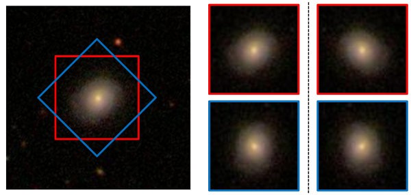
As mentioned before, the images were cropped to 207x207 and downsampled by a factor of 3. This was done with two different orientations: a regular crop, as well as one that is rotated 45°. Both of these crops were also flipped horizontally, resulting in four 69x69 “views” of the image. This is visualised below.

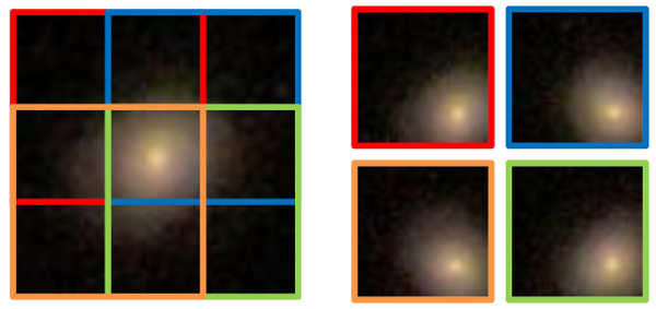
Each of the four views was again split into four partially overlapping “parts” of size 45x45. Each part was rotated so that they are all aligned, with the galaxy in the bottom right corner. This is visualised below. In total, 16 parts were extracted from the original image.

This results in 16 smaller 45x45 images which appear very similar. They can be expected to have the same topological structure due to rotation invariance, so they can be processed by the same convolutional architecture, which results in a 16x increase in parameter sharing, and thus less overfitting. At the top of the network, the features extracted from these 16 parts are concatenated and connected to one or more dense layers, so the information can be aggregated.
A nice side-effect of this approach is that the effective minibatch size for the convolutional part of the network increases 16-fold because the 16 parts are stacked on top of each other, which makes it easier to exploit GPU parallelism.
Due to the overlap of the parts, a lot of information is available about the center of the galaxy, because it is processed by the convnet in 16 different orientations. This is useful because a few important properties of the galaxies are expected to be in the center of the image (the presence of a bar or a bulge, for example). Reducing this overlap typically resulted in reduced performance. I chose not to make the parts fully overlap, because it would slow down training too much.
Incorporating output constraints
As described on this page, the 37 outputs to be predicted are weighted probabilities, adhering to a number of constraints. Incorporating these constraints into the model turned out to be quite useful.
In essence, the answers to each question should form a categorical distribution. Additionally, they are scaled by the probability of the question being asked, i.e. the total probability of answers given that would lead to this question being asked.
My initial reflex was to use a softmax output for each question, and then apply the scaling factors. This didn’t make much of a difference. I believe this is because the softmax function has difficulty predicting hard zeros and ones, of which there were quite a few in the training data (its input would have to be very large in magnitude).
If cross-entropy is the error metric, this is not a big issue, but for this competition, the metric by which submissions were judged was the root mean squared error (RMSE). As a result, being able to predict very low and very high probabilities was quite useful.
In the end I normalised the distribution for each question by adding a rectification nonlinearity in the top layer instead of the softmax functions, and then just using divisive normalisation. For example, if the raw, linear outputs of the top layer of the network for question one were z1, z2, z3, then the actual output for question one was given by max(z1, 0) / (max(z1, 0) + max(z2, 0) + max(z3, 0) + epsilon). The epsilon is a very small constant that prevented division by zero errors, I set it to 1e-12. This approach allowed the network to predict hard zeros more easily.
This is really where Theano shines: I could incorporate these constraints into the model simply by writing out what they were - no need to manually compute all the changed gradients. A big time saver! If I had to compute the gradients manually, I probably wouldn’t even have bothered to try incorporating the constraints in the first place.
Architecture of the best model
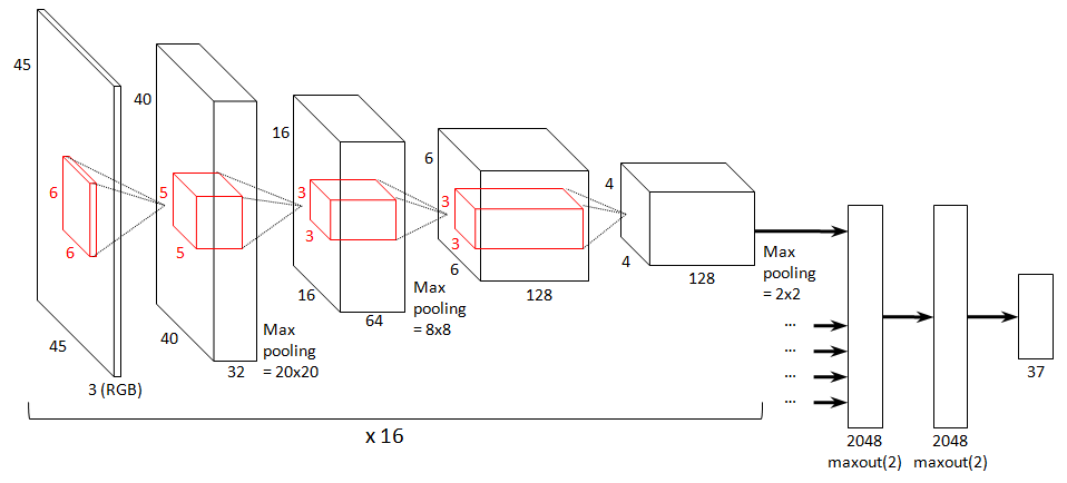
The best model I found is shown below in the form of a Krizhevsky-style diagram. All other models included in the final ensemble I submitted are slight variations of this model.

The input is presented to the model in the form of RGB coloured 45x45 image parts.
The model has 7 layers: 4 convolutional layers and 3 dense layers. All convolutional layers include a ReLU nonlinearity (i.e. f(x) = max(x, 0)). The first, second and fourth convolutional layers are followed by 2x2 max-pooling. The sizes of the layers, as well as the sizes of the filters, are indicated in the figure.
As mentioned before, the convolutional part of the network is applied to 16 different parts of the input image. The extracted features for all these parts are then aggregated and connected to the dense part of the network.
The dense part consists of two maxout layers with 2048 units (Goodfellow et al. 2013), both of which take the maximum over pairs of linear filters (so 4096 linear filters in total). Using maxout here instead of regular dense layers with ReLUs helped to reduce overfitting a lot, compared to dense layers with 4096 linear filters. Using maxout in the convolutional part of the network as well proved too computationally intensive.
Training this model took 67 hours.
Variants
Variants of the best model were included in the final ensemble I submitted, to increase variance (see “Model averaging”). They include:
- a network with two dense layers instead of three (just one maxout layer)
- a network with one of the dense layers reduced in size and applied individually to each part (resulting in 16-way parameter sharing for this layer as well)
- a network with a different filter size configuration: 8/4/3/3 instead of 6/5/3/3 (from bottom to top)
- a network with centered and rescaled input images
- a network with a ReLU dense layer instead of maxout
- a network with 192 filters instead of 128 for the topmost convolutional layer
- a network with 256 filters instead of 128 for the topmost convolutional layer
- a network with norm constraint regularisation applied to the two maxout layers (as in Hinton et al. 2012)
- combinations of the above variations
Training
Validation
For validation purposes, I split the training set in two parts. I used the first 90% for training, and the remainder for validation. I noticed quite early on that the estimates on my validation set matched the public leaderboard pretty well. This implied that submitting frequently was unnecessary - but nevertheless I couldn’t resist :)
Near the end of the competition I tried retraining a model on the entire training set, including the validation data I split off, but I noticed no increase in performance on the public leaderboard, so I left it at that. The separate validation set came in handy for model averaging anyway.
Training algorithm
I trained the networks with stochastic gradient descent (SGD) and Nesterov momentum (fixed at 0.9). I used a minibatch size of 16 examples. This meant that the effective minibatch size for the convolutional part was 256 (see above). This worked well because the cuda-convnet convolution implementation is optimised for minibatch sizes that are multiples of 128.
I trained the networks for about 1.5 million gradient steps. I used a learning rate schedule with two discrete decreases. Initially it was set to 0.04. It was decreased tenfold to 0.004 after about 1.1 million steps, and again to 0.0004 after about 1.4 million steps.
For the first ~600 gradient steps, the divisive normalisation in the output layer was disabled. This was necessary to ensure convergence (otherwise it would get stuck at the start sometimes).
Initialisation
Some fiddling with the parameter initialisation was required to get the network to train properly. Most of the layer weights were initialised from a Gaussian distribution with mean zero and a standard deviation of 0.01, with biases initialised to 0.1. For the topmost convolutional layer, I increased the standard deviation to 0.1. For the dense layers, I reduced it to 0.001 and the biases were initialised to 0.01. These modifications were necessary presumably because these layers are much smaller resp. bigger than the others.
Regularisation
Dropout was used in all three dense layers, with a dropout probability of 0.5. This was absolutely essential to be able to train the network at all.
Near the very end of the competition I also experimented with norm constraint regularisation for the maxout layers. I chose the maximal norm for each layer based on a histogram of the norms of a network trained without norm constraint regularisation (I chose it so the tail of the histogram would be chopped off). I’m not entirely sure if this helped or not, since I was only able to do two runs with this setup.
Model averaging
Averaging across transformed images
For each individual model, I computed predictions for 60 affine transformations of the test set images: a combination of 10 rotations, spaced by 36°, 3 rescalings (with scale factors 1/1.2, 1 and 1.2) and flipping / no flipping. These were uniformly averaged. Even though the model architecture already incorporated a lot of invariances, this still helped quite a bit.
Computing these averaged test set predictions for a single model took just over 4 hours.
Averaging across architectures
The averaged predictions for each model were then uniformly blended again, across a number of different models (variants of the model described under “Architecture of the best model”). I also experimented with a weighted blend, optimised on the validation set I split off, but this turned out not to make a significant difference. However, I did use the learned weights to identify sets of predictions that were not contributing at all, and I removed those from the uniform blend as well.
My final submission was a blend of predictions from 17 different models, each of which were themselves blended across 60 transformations of the input. So in the end, I blended 1020 predictions for each test set image.
For comparison: my best single model achieved a score of 0.07671 on the public leaderboard. After averaging, I achieved a final score of 0.7467. This resulted in a score of 0.07492 on the private leaderboard.
Miscellany
Below are a bunch of things that I tried but ended up not using - either because they didn’t help my score, or because they slowed down training too much.
- Adding Gaussian noise to the input images during training to reduce overfitting. This didn’t help.
- Extracting crops from the input images at different scales, and training a multiscale convnet on them. It turned out that only the part of the network for the most detailed scale was actually learning anything. The other parts received no gradient and weren’t really learning.
- Overlapping pooling. This seemed to help a little bit, but it slowed things down too much.
- Downsampling the input images less (1.5x instead of 3x) and using a strided convolution in the first layer (with stride 2). This did not improve results, and dramatically increased memory usage.
- Adding shearing to the data augmentation step. This didn’t help, but it didn’t hurt performance either. I assumed that it would hurt performance because question 7 pertains to the ellipticity of the galaxy (shearing would of course change this), but this didn’t seem to be the case.
Near the end of the competition I also toyed with a polar coordinate representation of the images. I suppose this could work well because rotations turn into translations in polar space, so the convnet’s inherent translation invariance would amount to rotation invariance in the original input space. Unfortunately I didn’t have enough time left to properly explore this approach, so I decided to focus on my initial approach instead.
I would also have liked to find a way to incorporate the test set images somehow (i.e. a transduction setup). Unsupervised pre-training seemed pointless, because it tends not to be beneficial when rectified linear units and dropout are used, except maybe when labeled training data is very scarce. I really like the pseudo-label approach of Dong-Hyun Lee (2013), but it could not be applied here because it only makes sense for classification problems, not regression problems. If anyone has ideas for this, I’m still interested!
Conclusion
This was a really cool competition, and even though I had some prior experience training convnets, I learnt a lot of new things about them.
If this problem interests you, be sure to check out the competition forum. Many of the participants will be posting overviews of their approaches in the coming days.
I would like to thank the organisers of the competition, as well as the authors of Theano, cuda-convnet and pylearn2 for providing me with the necessary tools.
I will clean up my code and I’ll put it on GitHub soon. If you have any questions or feedback about this post, feel free to leave a comment.
