Diffusion models appear to come in many shapes and forms. If you pick two random research papers about diffusion and look at how they describe the model class in their respective introductions, chances are they will go about it in very different ways. This can be both frustrating and enlightening: frustrating, because it makes it harder to spot relationships and equivalences across papers and implementations – but also enlightening, because these various perspectives each reveal new connections and are a breeding ground for new ideas. This blog post is an overview of the perspectives on diffusion I’ve found useful.

Last year, I wrote a blog post titled “diffusion models are autoencoders”. The title was tongue-in-cheek, but it highlighted a close connection between diffusion models and autoencoders, which I felt had been underappreciated up until then. Since so many more ML practitioners were familiar with autoencoders than with diffusion models, at the time, it seemed like a good idea to try and change that.

Since then, I’ve realised that I could probably write a whole series of blog posts, each highlighting a different perspective or equivalence. Unfortunately I only seem to be able to produce one or two blog posts a year, despite efforts to increase the frequency. So instead, this post will cover all of them at once in considerably less detail – but hopefully enough to pique your curiosity, or to make you see diffusion models in a new light.

This post will probably be most useful to those who already have at least a basic understanding of diffusion models. If you don’t count yourself among this group, or you’d like a refresher, check out my earlier blog posts on the topic:

• Diffusion models are autoencoders
• Guidance: a cheat code for diffusion models
• Diffusion language models

Before we start, a disclaimer: some of these connections are deliberately quite handwavy. They are intended to build intuition and understanding, and are not supposed to be taken literally, for the most part – this is a blog post, not a peer-reviewed research paper.

That said, I welcome any corrections and thoughts about the ways in which these equivalences don’t quite hold, or could even be misleading. Feel free to leave a comment, or reach out to me on Twitter (@sedielem) or Threads (@sanderdieleman). If you have a different perspective that I haven’t covered here, please share it as well.

Alright, here goes (click to scroll to each section):

1. Diffusion models are autoencoders
2. Diffusion models are deep latent variable models
3. Diffusion models predict the score function
4. Diffusion models solve reverse SDEs
5. Diffusion models are flow-based models
6. Diffusion models are recurrent neural networks
7. Diffusion models are autoregressive models
8. Diffusion models estimate expectations
9. Discrete and continuous diffusion models
10. Alternative formulations
11. Consistency
12. Defying conventions
13. Closing thoughts
14. Acknowledgements
15. References

Diffusion models are autoencoders

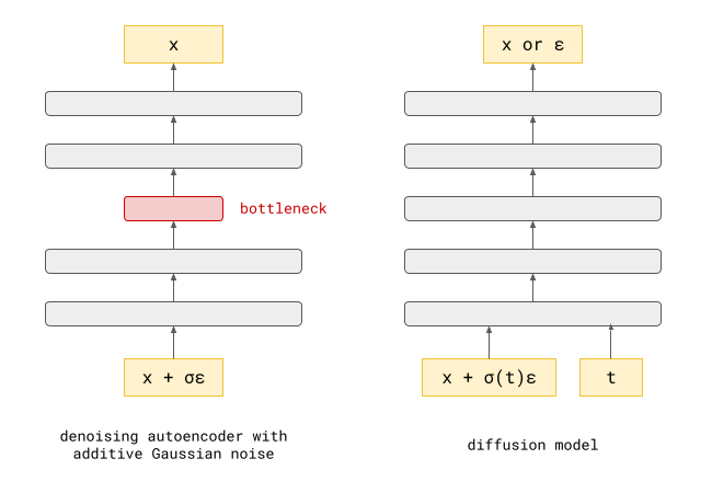
Denoising autoencoders are neural networks whose input is corrupted by noise, and they are tasked to predict the clean input, i.e. to remove the corruption. Doing well at this task requires learning about the distribution of the clean data. They have been very popular for representation learning, and in the early days of deep learning, they were also used for layer-wise pre-training of deep neural networks¹.

It turns out that the neural network used in a diffusion model usually solves a very similar problem: given an input example corrupted by noise, it predicts some quantity associated with the data distribution. This can be the corresponding clean input (as in denoising autoencoders), the noise that was added, or something in between (more on that later). All of these are equivalent in some sense when the corruption process is linear, i.e., the noise is additive: we can turn a model that predicts the noise into a model that predicts the clean input, simply by subtracting its prediction from the noisy input. In neural network parlance, we would be adding a residual connection from the input to the output.

There are a few key differences:

• Denoising autoencoders often have some sort of information bottleneck somewhere in the middle, to learn a useful representation of the input whose capacity is constrained in some way. The denoising task itself is merely a means to an end, and not what we actually want to use the models for once we’ve trained them. The neural networks used for diffusion models don’t typically have such a bottleneck, as we are more interested in their predictions, rather than the internal representations they construct along the way to be able to make those predictions.

• Denoising autoencoders can be trained with a variety of types of noise. For example, parts of the input could be masked out (masking noise), or we could add noise drawn from some arbitrary distribution (often Gaussian). For diffusion models, we usually stick with additive Gaussian noise because of its helpful mathematical properties, which simplify a lot of operations.

• Another important difference is that denoising autoencoders are usually trained to deal only with noise of a particular strength. In a diffusion model, we have to be able to make predictions for inputs with a lot of noise, or with very little noise. The noise level is provided to the neural network as an extra input.

As mentioned, I’ve already discussed this relationship in detail in a previous blog post, so check that out if you are keen to explore this connection more thoroughly.

Diffusion models are deep latent variable models

Sohl-Dickstein et al. first suggested using a diffusion process to gradually destroy structure in data, and then constructing a generative model by learning to reverse this process in a 2015 ICML paper². Five years later, Ho et al. built on this to develop Denoising Diffusion Probabilistic Models or DDPMs³, which formed the blueprint of modern diffusion models along with score-based models (see below).

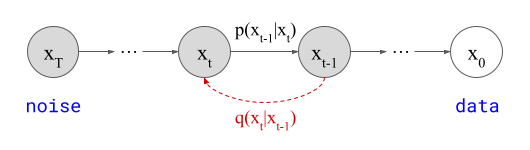
In this formulation, represented by the graphical model above, \(\mathbf{x}_T\) (latent) represents Gaussian noise and \(\mathbf{x}_0\) (observed) represents the data distribution. These random variables are bridged by a finite number of intermediate latent variables \(\mathbf{x}_t\) (typically \(T=1000\)), which form a Markov chain, i.e. \(\mathbf{x}_{t-1}\) only depends on \(\mathbf{x}_t\), and not directly on any preceding random variables in the chain.

The parameters of the Markov chain are fit using variational inference to reverse a diffusion process, which is itself a Markov chain (in the other direction, represented by \(q(\mathbf{x}_t \mid \mathbf{x}_{t-1})\) in the diagram) that gradually adds Gaussian noise to the data. Concretely, as in Variational Autoencoders (VAEs)⁴⁵, we can write down an Evidence Lower Bound (ELBO), a bound on the log likelihood, which we can maximise tractably. In fact, this section could just as well have been titled “diffusion models are deep VAEs”, but I’ve already used “diffusion models are autoencoders” for a different perspective, so I figured this might have been a bit confusing.

We know \(q(\mathbf{x}_t \mid \mathbf{x}_{t-1})\) is Gaussian by construction, but \(p(\mathbf{x}_{t-1} \mid \mathbf{x}_t)\), which we are trying to fit with our model, need not be! However, as long as each individual step is small enough (i.e. \(T\) is large enough), it turns out that we can parameterise \(p(\mathbf{x}_{t-1} \mid \mathbf{x}_t)\) as if it were Gaussian, and the approximation error will be small enough for this model to still produce good samples. This is kind of surprising when you think about it, as during sampling, any errors may accumulate over \(T\) steps.

Full disclosure: out of all the different perspectives on diffusion in this blog post, this is probably the one I understand least well. Sort of ironic, given how popular it is, but variational inference has always been a little bit mysterious to me. I will stop here, and mostly defer to a few others who have described this perspective in detail (apart from the original DDPM paper, of course):

• “Diffusion Models as a kind of VAE” by Angus Turner
• Jakub Tomczak’s blog post on DDPMs
• Lilian Weng’s blog post on diffusion models (connects multiple perspectives)
• Alex Alemi’s blog post about the variational diffusion loss

Diffusion models predict the score function

Most likelihood-based generative models parameterise the log-likelihood of an input \(\mathbf{x}\), \(\log p(\mathbf{x} \mid \theta)\), and then fit the model parameters \(\theta\) to maximise it, either approximately (as in VAEs) or exactly (as in flow-based models or autoregressive models). Because log-likelihoods represent probability distributions, and probability distributions have to be normalised, this usually requires some constraints to ensure all possible values for the parameters \(\theta\) yield valid distributions. For example, autoregressive models have causal masking to ensure this, and most flow-based models require invertible neural network architectures.

It turns out there is another way to fit distributions that neatly sidesteps this normalisation requirement, called score matching⁶. It’s based on the observation that the so-called score function, \(s_\theta(\mathbf{x}) := \nabla_\mathbf{x} \log p(\mathbf{x} \mid \theta)\), is invariant to the scaling of \(p(\mathbf{x} \mid \theta)\). This is easy to see:

Any arbitrary scale factor applied to the probability density simply disappears. Therefore, if we have a model that parameterises a score estimate \(\hat{s}_\theta(\mathbf{x})\) directly, we can fit the distribution by minimising the score matching loss (instead of maximising the likelihood directly):

In this form however, this loss function is not practical, because we do not have a good way to compute ground truth scores \(\nabla_\mathbf{x} \log p(\mathbf{x})\) for any data point \(\mathbf{x}\). There are a few tricks that can be applied to sidestep this requirement, and transform this into a loss function that’s easy to compute, including implicit score matching (ISM)⁶, sliced score matching (SSM)⁷ and denoising score matching (DSM)⁸. We’ll take a closer look at this last one:

Here, \(\tilde{\mathbf{x}}\) is obtained by adding Gaussian noise to \(\mathbf{x}\). This means \(p(\tilde{\mathbf{x}} \mid \mathbf{x})\) is distributed according to a Gaussian distribution \(\mathcal{N}\left(\mathbf{x}, \sigma^2\right)\) and the ground truth conditional score function can be calculated in closed form:

This form has a very intuitive interpretation: it is a scaled version of the Gaussian noise added to \(\mathbf{x}\) to obtain \(\tilde{\mathbf{x}}\). Therefore, making \(\tilde{\mathbf{x}}\) more likely by following the score (= gradient ascent on the log-likelihood) directly corresponds to removing (some of) the noise:

If we choose the step size \(\eta = \sigma^2\), we recover the clean data \(\mathbf{x}\) in a single step.

\(\mathcal{L}_{SM}\) and \(\mathcal{L}_{DSM}\) are different loss functions, but the neat thing is that they have the same minimum in expectation: \(\mathbb{E}_\mathbf{x} [\mathcal{L}_{SM}] = \mathbb{E}_{\mathbf{x},\tilde{\mathbf{x}}} [\mathcal{L}_{DSM}] + C\), where \(C\) is some constant. Pascal Vincent derived this equivalence back in 2010 (before score matching was cool!) and I strongly recommend reading his tech report about it⁸ if you want to deepen your understanding.

One important question this approach raises is: how much noise should we add, i.e. what should \(\sigma\) be? Picking a particular fixed value for this hyperparameter doesn’t actually work very well in practice. At low noise levels, it is very difficult to estimate the score accurately in low-density regions. At high noise levels, this is less of a problem, because the added noise spreads out the density in all directions – but then the distribution that we’re modelling is significantly distorted by the noise. What works well is to model the density at many different noise levels. Once we have such a model, we can anneal \(\sigma\) during sampling, starting with lots of noise and gradually dialing it down. Song & Ermon describe these issues and their elegant solution in detail in their 2019 paper⁹.

This combination of denoising score matching at many different noise levels with gradual annealing of the noise during sampling yields a model that’s essentially equivalent to a DDPM, but the derivation is completely different – no ELBOs in sight! To learn more about this perspective, check out Yang Song’s excellent blog post on the topic.

Diffusion models solve reverse SDEs

In both of the previous perspectives (deep latent variable models and score matching), we consider a discete and finite set of steps. These steps correspond to different levels of Gaussian noise, and we can write down a monotonic mapping \(\sigma(t)\) which maps the step index \(t\) to the standard deviation of the noise at that step.

If we let the number of steps go to infinity, it makes sense to replace the discrete index variable with a continuous value \(t\) on an interval \([0, T]\), which can be interpreted as a time variable, i.e. \(\sigma(t)\) now describes the evolution of the standard deviation of the noise over time. In continuous time, we can describe the diffusion process which gradually adds noise to data points \(\mathbf{x}\) with a stochastic differential equation (SDE):

This equation relates an infinitesimal change in \(\mathbf{x}\) with an infintesimal change in \(t\), and \(\mathrm{d}\mathbf{w}\) represents infinitesimal Gaussian noise, also known as the Wiener process. \(\mathbf{f}\) and \(g\) are called the drift and diffusion coefficients respectively. Particular choices for \(\mathbf{f}\) and \(g\) yield time-continuous versions of the Markov chains used to formulate DDPMs.

SDEs combine differential equations with stochastic random variables, which can seem a bit daunting at first. Luckily we don’t need too much of the advanced SDE machinery that exists to understand how this perspective can be useful for diffusion models. However, there is one very important result that we can make use of. Given an SDE that describes a diffusion process like the one above, we can write down another SDE that describes the process in the other direction, i.e. reverses time¹⁰:

This equation also describes a diffusion process. \(\mathrm{d}\bar{\mathbf{w}}\) is the reversed Wiener process, and \(\nabla_\mathbf{x} \log p_t(\mathbf{x})\) is the time-dependent score function. The time dependence comes from the fact that the noise level changes over time.

Explaining why this is the case is beyond the scope of this blog post, but the original paper by Yang Song and colleagues that introduced the SDE-based formalism for diffusion models¹¹ is well worth a read.

Concretely, if we have a way to estimate the time-dependent score function, we can simulate the reverse diffusion process, and therefore draw samples from the data distribution starting from noise. So we can once again train a neural network to predict this quantity, and plug it into the reverse SDE to obtain a continuous-time diffusion model.

In practice, simulating this SDE requires discretising the time variable \(t\) again, so you might wonder what the point of all this is. What’s neat is that this discretisation is now something we can decide at sampling-time, and it does not have to be fixed before we train our score prediction model. In other words, we can trade off sample quality for computational cost in a very natural way without changing the model, by choosing the number of sampling steps.

Diffusion models are flow-based models

Remember flow-based models^{12 13}? They aren’t very popular for generative modelling these days, which I think is mainly because they tend to require more parameters than other types of models to achieve the same level of performance. This is due to their limited expressivity: neural networks used in flow-based models are required to be invertible, and the log-determinant of the Jacobian must be easy to compute, which imposes significant constraints on the kinds of computations that are possible.

At least, this is the case for discrete normalising flows. Continuous normalising flows (CNFs)^{14 15} also exist, and usually take the form of an ordinary differential equation (ODE) parameterised by a neural network, which describes a deterministic path between samples from the data distribution and corresponding samples from a simple base distribution (e.g. standard Gaussian). CNFs are not affected by the aforementioned neural network architecture constraints, but in their original form, they require backpropagation through an ODE solver to train. Although some tricks exist to do this more efficiently, this probably also presents a barrier to widespread adoption.

Let’s revisit the SDE formulation of diffusion models, which describes a stochastic process mapping samples from a simple base distribution to samples from the data distribution. An interesting question to ask is: what does the distribution of the intermediate samples \(p_t(\mathbf{x})\) look like, and how does it evolve over time? This is governed by the so-called Fokker-Planck equation. If you want to see what this looks like in practice, check out appendix D.1 of Song et al. (2021)¹¹.

Here’s where it gets wild: there exists an ODE that describes a deterministic process whose time-dependent distributions are exactly the same as those of the stochastic process described by the SDE. This is called the probability flow ODE. What’s more, it has a simple closed form:

This equation describes both the forward and backward process (just flip the sign to go in the other direction), and note that the time-dependent score function \(\nabla_\mathbf{x} \log p_t(\mathbf{x})\) once again features. To prove this, you can write down the Fokker-Planck equations for both the SDE and the probability flow ODE, and do some algebra to show that they are the same, and hence must have the same solution \(p_t(\mathbf{x})\).

Note that this ODE does not describe the same process as the SDE: that would be impossible, because a deterministic differential equation cannot describe a stochastic process. Instead, it describes a different process with the unique property that the distributions \(p_t(\mathbf{x})\) are the same for both processes. Check out the probability flow ODE section in Yang Song’s blog post for a great diagram comparing both processes.

The implications of this are profound: there is now a bijective mapping between particular samples from the simple base distribution, and samples from the data distribution. We have a sampling process where all the randomness is contained in the initial base distribution sample – once that’s been sampled, going from there to a data sample is completely deterministic. It also means that we can map data points to their corresponding latent representations by simulating the ODE forward, manipulating them, and then mapping them back to the data space by simulating the ODE backward.

The model described by the probability flow ODE is a continuous normalising flow, but it’s one that we managed to train without having to backpropagate through an ODE, rendering the approach much more scalable.

The fact that all this is possible, without even changing anything about how the model is trained, still feels like magic to me. We can plug our score predictor into the reverse SDE from the previous section, or the ODE from this one, and get out two different generative models that model the same distribution in different ways. How cool is that?

As a bonus, the probability flow ODE also enables likelihood computation for diffusion models (see appendix D.2 of Song et al. (2021)¹¹). This also requires solving the ODE, so it’s roughly as expensive as sampling.

For all of the reasons above, the probability flow ODE paradigm has proven quite popular recently. Among other examples, it is used by Karras et al.¹⁶ as a basis for their work investigating various diffusion modelling design choices, and my colleagues and I recently used it for our work on diffusion language models¹⁷. It has also been generalised and extended beyond diffusion processes, to enable learning a mapping between any pair of distributions, e.g. in the form of Flow Matching¹⁸, Rectified Flows¹⁹ and Stochastic Interpolants²⁰.

Side note: another way to obtain a deterministic sampling process for diffusion models is given by DDIM²¹, which is based on the deep latent variable model perspective.

Diffusion models are recurrent neural networks (RNNs)

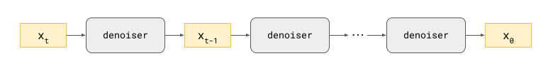
Sampling from a diffusion model involves making repeated predictions with a neural network and using those predictions to update a canvas, which starts out filled with random noise. If we consider the full computational graph of this process, it starts to look a lot like a recurrent neural network (RNN). In RNNs, there is a hidden state which repeatedly gets updated by passing it through a recurrent cell, which consists of one or more nonlinear parameterised operations (e.g. the gating mechanisms of LSTMs²²). Here, the hidden state is the canvas, so it lives in the input space, and the cell is formed by the denoiser neural network that we’ve trained for our diffusion model.

RNNs are usually trained with backpropagation through time (BPTT), with gradients propagated through the recurrence. The number of recurrent steps to backpropagate through is often limited to some maximum number to reduce the computational cost, which is referred to as truncated BPTT. Diffusion models are also trained by backpropagation, but only through one step at a time. In some sense, diffusion models present a way to train deep recurrent neural networks without backpropagating through the recurrence at all, yielding a much more scalable training procedure.

RNNs are usually deterministic, so this analogy makes the most sense for the deterministic process based on the probability flow ODE described in the previous section – though injecting noise into the hidden state of RNNs as a means of regularisation is not unheard of, so I think the analogy also works for the stochastic process.

The total depth of this computation graph in terms of the number of nonlinear layers is given by the number of layers in our neural network, multiplied by the number of sampling steps. We can look at the unrolled recurrence as a very deep neural network in its own right, with potentially thousands of layers. This is a lot of depth, but it stands to reason that a challenging task like generative modelling of real-world data requires such deep computation graphs.

We can also consider what happens if we do not use the same neural network at each diffusion sampling step, but potentially different ones for different ranges of noise levels. These networks can be trained separately and independently, and can even have different architectures. This means we are effectively “untying the weights” in our very deep network, turning it from an RNN into a plain old deep neural network, but we are still able to avoid having to backpropagate through all of it in one go. Stable Diffusion XL²³ uses this approach to great effect for its “Refiner” model, so I think it might start to catch on.

When I started my PhD in 2010, training neural networks with more than two hidden layers was a chore: backprop didn’t work well out of the box, so we used unsupervised layer-wise pre-training^{1 24} to find a good initialisation which would make backpropagation possible. Nowadays, even hundreds of nonlinear layers do not form an obstacle anymore. Therefore it’s not inconceivable that several years from now, training networks with tens of thousands of layers by backprop will be within reach. At that point, the “divide and conquer” approach that diffusion models offer might lose its luster, and perhaps we’ll all go back to training deep variational autoencoders! (Note that the same “divide and conquer” perspective equally applies to autoregressive models, so they would become obsolete as well, in that case.)

One question this perspective raises is whether diffusion models might actually work better if we backpropagated through the sampling procedure for two or more steps. This approach isn’t popular, which probably indicates that it isn’t cost-effective in practice. There is one important exception (sort of): models which use self-conditioning²⁵, such as Recurrent Interface Networks (RINs)²⁶, pass some form of state between the diffusion sampling steps, in addition to the updated canvas. To enable the model to learn to make use of this state, an approximation of it is made available during training by running an additional forward pass. There is no additional backward pass though, so this doesn’t really count as two steps of BPTT – more like 1.5 steps.

Diffusion models are autoregressive models

For diffusion models of natural images, the sampling process tends to produce large-scale structure first, and then iteratively adds more and more fine-grained details. Indeed, there seems to be almost a direct correspondence between noise levels and feature scales, which I discussed in more detail in Section 5 of a previous blog post.

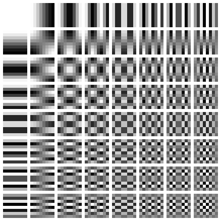
But why is this the case? To understand this, it helps to think in terms of spatial frequencies. Large-scale features in images correspond to low spatial frequencies, whereas fine-grained details correspond to high frequencies. We can decompose images into their spatial frequency components using the 2D Fourier transform (or some variant of it). This is often the first step in image compression algorithms, because the human visual system is known to be much less sensitive to high frequencies, and this can be exploited by compressing them more aggressively than low frequencies.

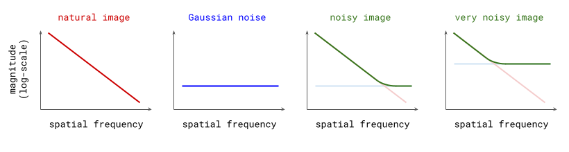
Natural images, along with many other natural signals, exhibit an interesting phenomenon in the frequency domain: the magnitude of different frequency components tends to drop off proportionally to the inverse of the frequency²⁷: \(S(f) \propto 1/f\) (or the inverse of the square of the frequency, if you’re looking at power spectra instead of magnitude spectra).

Gaussian noise, on the other hand, has a flat spectrum: in expectation, all frequencies have the same magnitude. Since the Fourier transform is a linear operation, adding Gaussian noise to a natural image yields a new image whose spectrum is the sum of the spectrum of the original image, and the flat spectrum of the noise. In the log-domain, this superposition of the two spectra looks like a hinge, which shows how the addition of noise obscures any structure present in higher spatial frequencies (see figure below). The larger the standard deviation of this noise, the more spatial frequencies will be affected.

Since diffusion models are constructed by progressively adding more noise to input examples, we can say that this process increasingly drowns out lower and lower frequency content, until all structure is erased (for natural images, at least). When sampling from the model, we go in the opposite direction and effectively add structure at higher and higher spatial frequencies. This basically looks like autoregression, but in frequency space! Rissanen et al. (2023) discuss this observation in Section 2.2 of their paper²⁸ on generative modelling with inverse heat dissipation (as an alternative to Gaussian diffusion), though they do not make the connection to autoregressive models. I added that bit, so this section could have a provocative title.

An important caveat is that this interpretation relies on the frequency characteristics of natural signals, so for applications of diffusion models in other domains (e.g. language modelling, see Section 2 of my blog post on diffusion language models), the analogy may not make sense.

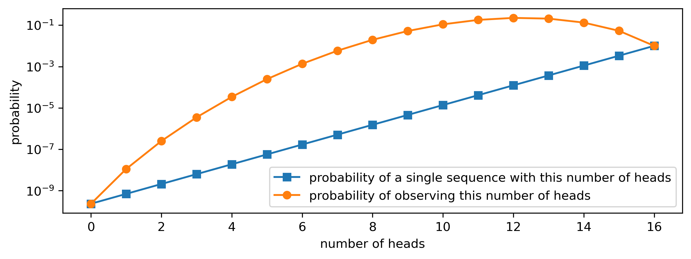
Diffusion models estimate expectations

Consider the transition density \(p(\mathbf{x}_t \mid \mathbf{x}_0)\), which describes the distribution of the noisy data example \(\mathbf{x}_t\) at time \(t\), conditioned on the original clean input \(\mathbf{x}_0\) it was derived from (by adding noise). Based on samples from this distribution, the neural network used in a diffusion model is tasked to predict the expectation \(\mathbb{E}[\mathbf{x}_0 \mid \mathbf{x}_t]\) (or some linear time-dependent function of it). This may seem a tad obvious, but I wanted to highlight some of the implications.

First, it provides another motivation for why the mean squared error (MSE) is the right loss function to use for training diffusion models. During training, the expectation \(\mathbb{E}[\mathbf{x}_0 \mid \mathbf{x}_t]\) is not known, so instead we supervise the model using \(\mathbf{x}_0\) itself. Because the minimiser of the MSE loss is precisely the expectation, we end up recovering (an approximation of) \(\mathbb{E}[\mathbf{x}_0 \mid \mathbf{x}_t]\), even though we don’t know this quantity a priori. This is a bit different from typical supervised learning problems, where the ideal outcome would be for the model to predict exactly the targets used to supervise it (barring any label errors). Here, we purposely do not want that. More generally, the notion of being able to estimate conditional expectations, even though we only provide supervision through samples, is very powerful.

Second, it explains why distillation²⁹ of diffusion models^{30 31 32} is such a compelling proposition: in this setting, we are able to supervise a diffusion model directly with an approximation of the target expectation \(\mathbb{E}[\mathbf{x}_0 \mid \mathbf{x}_t]\) that we want it to predict, because that is what the teacher model already provides. As a result, the variance of the training loss will be much lower than if we had trained the model from scratch, and convergence will be much faster. Of course, this is only useful if you already have a trained model on hand to use as a teacher.

Discrete and continuous diffusion models

So far, we have covered several perspectives that consider a finite set of discrete noise levels, and several perspectives that use a notion of continuous time, combined with a mapping function \(\sigma(t)\) to map time steps to the corresponding standard deviation of the noise. These are typically referred to as discrete-time and continuous-time respectively. One thing that’s quite neat is that this is mostly a matter of interpretation: models trained within a discrete-time perspective can usually be repurposed quite easily to work in the continuous-time setting¹⁶, and vice versa.

Another way in which diffusion models can be discrete or continuous, is with respect to the input space. In the literature, I’ve found that it is sometimes unclear whether “continuous” or “discrete” are meant to be with respect to time, or with respect to the input. This is especially important because some perspectives only really make sense for continuous input, as they rely on gradients with respect to the input (i.e. all perspectives based on the score function).

All four combinations of discreteness/continuity exist:

• discrete time, continuous input: the original deep latent variable model perspective (DDPMs), as well as the score-based perspective;
• continuous time, continuous input: SDE- and ODE-based perspectives;
• discrete time, discrete input: D3PM³³, MaskGIT³⁴, Mask-predict³⁵, ARDM³⁶, Multinomial diffusion³⁷ and SUNDAE³⁸ are all methods that use iterative refinement on discrete inputs – whether all of these should be considered diffusion models isn’t entirely clear (it depends on who you ask);
• continuous time, discrete input: Continuous Time Markov Chains (CTMCs)³⁹, Score-based Continuous-time Discrete Diffusion Models⁴⁰ and Blackout Diffusion⁴¹ all pair discrete input with continuous time – this setting is also often handled by embedding discrete data in Euclidean space, and then performing input-continuous diffusion in that space, as in e.g. Analog Bits²⁵, Self-conditioned Embedding Diffusion⁴² and CDCD¹⁷.

Alternative formulations

Recently, a few papers have proposed new derivations of this class of models from first principles with the benefit of hindsight, avoiding concepts such as differential equations, ELBOs or score matching altogether. These works provide yet another perspective on diffusion models, which may be more accessible because it requires less background knowledge.

Inversion by Direct Iteration (InDI)⁴³ is a formulation rooted in image restoration, intended to harness iterative refinement to improve perceptual quality. No assumptions are made about the nature of the image degradations, and models are trained on paired low-quality and high-quality examples. Iterative \(\alpha\)-(de)blending⁴⁴ uses linear interpolation between samples from two different distributions as a starting point to obtain a deterministic mapping between the distributions. Both of these methods are also closely related to Flow Matching¹⁸, Rectified Flow¹⁹ and Stochastic Interpolants²⁰ discussed earlier.

Consistency

A few different notions of “consistency” in diffusion models have arisen in literature recently:

• Consistency models (CM)⁴⁵ are trained to map points on any trajectory of the probability flow ODE to the trajectory’s origin (i.e. the clean data point), enabling sampling in a single step. This is done indirectly by taking pairs of points on a particular trajectory and ensuring that the model output is the same for both (hence “consistency”). There is a distillation variant which starts from an existing diffusion model, but it is also possible to train a consistency model from scratch.

• Consistent diffusion models (CDM)⁴⁶ are trained using a regularisation term that explicitly encourages consistency, which they define to mean that the prediction of the denoiser should correspond to the conditional expectation \(\mathbb{E}[\mathbf{x}_0 \mid \mathbf{x}_t]\) (see earlier).

• FP-Diffusion⁴⁷ takes the Fokker-Planck equation describing the evolution across time of \(p_t(\mathbf{x})\), and introduces an explicit regularisation term to ensure that it holds.

Each of these properties would trivially hold for an ideal diffusion model (i.e. fully converged, in the limit of infinite capacity). However, real diffusion models are approximate, and so they tend not to hold in practice, which is why it makes sense to add mechanisms to explicitly enforce them.

The main reason for including this section here is that I wanted to highlight a recent paper by Lai et al. (2023)⁴⁸ that shows that these three different notions of consistency are essentially different perspectives on the same thing. I thought this was a very elegant result, and it definitely suits the theme of this blog post!

Defying conventions

Apart from all these different perspectives on a conceptual level, the diffusion literature is also particularly fraught in terms of reinventing notation and defying conventions, in my experience. Sometimes, even two different descriptions of the same conceptual perspective look nothing alike. This doesn’t help accessibility and increases the barrier to entry. (I’m not blaming anyone for this, to be clear – in fact, I suspect I might be contributing to the problem with this blog post. Sorry about that.)

There are also a few other seemingly innocuous details and parameterisation choices that can have profound implications. Here are three things to watch out for:

• By and large, people use variance-preserving (VP) diffusion processes, where in addition to adding noise at each step, the current canvas is rescaled to preserve the overall variance. However, the variance-exploding (VE) formulation, where no rescaling happens and the variance of the added noise increases towards infinity, has also gained some followers. Most notably it is used by Karras et al. (2022)¹⁶. Some results that hold for VP diffusion might not hold for VE diffusion or vice versa (without making the requisite changes), and this might not be mentioned explicitly. If you’re reading a diffusion paper, make sure you are aware of which formulation is used, and whether any assumptions are being made about it.

• Sometimes, the neural network used in a diffusion model is parameterised to predict the (standardised) noise added to the input, or the score function; sometimes it predicts the clean input instead, or even a time-dependent combination of the two (as in e.g. \(\mathbf{v}\)-prediction³⁰). All of these targets are equivalent in the sense that they are time-dependent linear functions of each other and the noisy input \(\mathbf{x}_t\). But it is important to understand how this interacts with the relative weighting of loss contributions for different time steps during training, which can significantly affect model performance. Out of the box, predicting the standardised noise seems to be a great choice for image data. When modelling certain other quantities (e.g. latents in latent diffusion), people have found predicting the clean input to work better. This is primarily because it implies a different weighting of noise levels, and hence feature scales.

• It is generally understood that the standard deviation of the noise added by the corruption process increases with time, i.e. entropy increases over time, as it tends to do in our universe. Therefore, \(\mathbf{x}_0\) corresponds to clean data, and \(\mathbf{x}_T\) (for some large enough \(T\)) corresponds to pure noise. Some works (e.g. Flow Matching¹⁸) invert this convention, which can be very confusing if you don’t notice it straight away.

Finally, it’s worth noting that the definition of “diffusion” in the context of generative modelling has grown to be quite broad, and is now almost equivalent to “iterative refinement”. A lot of “diffusion models” for discrete input are not actually based on diffusion processes, but they are of course closely related, so the scope of this label has gradually been extended to include them. It’s not clear where to draw the line: if any model which implements iterative refinement through inversion of a gradual corruption process is a diffusion model, then all autoregressive models are also diffusion models. To me, that seems confusing enough so as to render the term useless.

Closing thoughts

Learning about diffusion models right now must be a pretty confusing experience, but the exploration of all these different perspectives has resulted in a diverse toolbox of methods which can all be combined together, because ultimately, the underlying model is always the same. I’ve also found that learning about how the different perspectives relate to each other has considerably deepened my understanding. Some things that are a mystery from one perspective are clear as day in another.

If you are just getting started with diffusion, hopefully this post will help guide you towards the right things to learn next. If you are a seasoned diffuser, I hope I’ve broadened your perspectives and I hope you’ve learnt something new nevertheless. Thanks for reading!

What's your favourite perspective on diffusion? Are there any useful perspectives that I've missed? Please share your thoughts in the comments below, or reach out on Twitter (@sedielem) or Threads (@sanderdieleman) if you prefer. Email is okay too.

I will also be at ICML 2023 in Honolulu and would be happy to chat in person!

If you would like to cite this post in an academic context, you can use this BibTeX snippet:

@misc{dieleman2023perspectives,
  author = {Dieleman, Sander},
  title = {Perspectives on diffusion},
  url = {https://sander.ai/2023/07/20/perspectives.html},
  year = {2023}
}

Acknowledgements

Thanks to my colleagues at Google DeepMind for various discussions, which continue to shape my thoughts on this topic! Thanks to Ayan Das, Ira Korshunova, Peyman Milanfar, and Çağlar Ünlü for suggestions and corrections.

References

Diffusion models have completely taken over generative modelling of perceptual signals such as images, audio and video. Why is autoregression still the name of the game for language modelling? And can we do anything about that? Some thoughts about what it will take for other forms of iterative refinement to take over language modelling, the last bastion of autoregression.

The rise of diffusion models

Roughly three years ago, things were starting to look as if adversarial image generators were about to be supplanted by a powerful combination of autoregression and discrete representation learning. BigGAN¹ and StyleGAN² had significantly expanded the capabilities of image generators, but the mode-seeking nature of GANs made them favour realism over diversity. This presented some challenges, and people were having trouble reproducing impressive domain-specific results (e.g. generating realistic human faces) on more diverse training datasets.

VQ-VAE 2³ and especially VQGAN⁴ extolled the virtue of a two-stage approach to generative modelling: first turn everything into a highly compressed discrete one-dimensional sequence, and then learn to predict this sequence step-by-step using a powerful autoregressive model. This idea had already proven fruitful before, going back to the original VQ-VAE⁵, but these two papers really drove the point home that this was our best bet for generative modelling of diverse data at scale.

But then, a challenger appeared: a new generative modelling approach based on iterative denoising was starting to show promise. Yang Song and Stefano Ermon proposed score-based models: while their NeurIPS 2019 paper⁶ was more of a proof-of-concept, the next year’s follow-up ‘Improved Techniques for Training Score-Based Generative Models’⁷ showed results that convinced some people (including me!) to take this direction of research more seriously. Another NeurIPS 2020 paper by Jonathan Ho, Ajay Jain and Pieter Abbeel, ‘Denoising Diffusion Probabilistic Models’ (DDPMs)⁸ showed similar results, and it didn’t take people too long to realise that DDPMs and score-based models were two sides of the same coin.

The real triumph of diffusion models over other alternatives for image generation came in 2021, with ‘Diffusion Models Beat GANs on Image Synthesis’⁹ by Prafulla Dhariwal and Alex Nichol. At that point, it was pretty clear to everyone in the know that this approach was poised to take over. Powerful diffusion-based text-to-image models such as GLIDE¹⁰ started to arrive by the end of that year, and proceeded to go mainstream in 2022.

If you are unfamiliar with diffusion models, I recommend reading at least the first section of my previous blog post ‘Diffusion models are autoencoders’ for context, before reading the rest of this one.

Diffusion for images: a match made in heaven

Diffusion models and the human visual system have one important thing in common: they don’t care too much about high frequencies. At least, not out of the box. I discussed the reasons for this in some detail in an earlier blog post (section 5 in particular).

In a nutshell, the different levels of noise at which a diffusion model operates allow it to focus on different spatial frequency components of the image at each iterative refinement step. When sampling an image, the model effectively builds it up from low frequencies to high frequencies, first filling in large-scale structure and then adding progressively more fine-grained details.

During training, we sample a noise level for each training example, add noise to it, and then try to predict the noise. The relative weights with which we sample the different noise levels therefore determine the degree to which the model focuses on large-scale and fine-grained structure. The most commonly used formulation, with uniform weighting of the noise levels, yields a very different objective than the likelihood loss which e.g. autoregressive models are trained with.

It turns out that there is a particular weighting which corresponds directly to the likelihood loss¹¹, but this puts significantly more weight on very low noise levels. Since low noise levels correspond to high spatial frequencies, this also indirectly explains why likelihood-based autoregressive models in pixel space never really took off: they end up spending way too much of their capacity on perceptually meaningless detail, and never get around to modelling larger-scale structure.

Relative to the likelihood loss, uniform weighting across noise levels in diffusion models yields an objective that is much more closely aligned with the human visual system. I don’t believe this was actually known when people first started training diffusion models on images – it was just a lucky coincidence! But we understand this pretty well now, and I think it is one of the two main reasons why this modelling approach completely took over in a matter of two years. (The other reason is of course classifier-free guidance, which you can read more about in my previous blog post on the topic.)

The reason I bring all this up here, is that it doesn’t bode particularly well for applications of diffusion models beyond the perceptual domain. Our ears have a similar disdain for high frequencies as our eyes (though to a lesser extent, I believe), but in the language domain, what does “high frequency” even mean¹²? Given the success of likelihood-based language models, could the relatively lower weight of low noise levels actually prove to be a liability in this setting?

Autoregression for language: a tough baseline to beat

Autoregression at the word or token level is a very natural way to do language modelling, because to some degree, it reflects how language is produced and consumed: as a one-dimensional sequence, one element at a time, in a particular fixed order. However, if we consider the process through which an abstract thought turns into an utterance, the iterative denoising metaphor starts to look more appealing. When writing a paragraph, the core concepts are generally decided on first, and the exact wording and phrasing doesn’t materialise until later. That said, perhaps it doesn’t matter precisely how humans interact with language: just like how planes don’t fly the same way birds do (h/t Yann LeCun), the best way to build a practically useful language model need not reflect nature either.

Practically speaking, autoregressive models have an interface that is somewhat limited: they can be prompted, i.e. tasked to complete a sequence for which a prefix is given. While this has actually been shown to be reasonably versatile in itself, the ability of non-autoregressive models to fill in the blanks (i.e. be conditioned on something other than a prefix, also known as inpainting in the image domain) is potentially quite useful, and not something that comes naturally to autoregressive models (though it is of course possible to do infilling with autoregressive models¹³).

Training efficiency

If we compare autoregression and diffusion side-by-side as different forms of iterative refinement, the former has the distinct advantage that training can be parallelised trivially across all refinement steps. During autoregressive model training, we obtain a useful gradient signal from all steps in the sampling process. This is not true for diffusion models, where we have to sample a particular noise level for each training example. It is not practical to train on many different noise levels for each example, because that would require multiple forward and backward passes through the model. For autoregression, we get gradients for all sequence steps with just a single forward-backward pass.

As a result, diffusion model training is almost certainly significantly less statistically efficient than autoregressive model training, and slower convergence implies higher computational requirements.

Sampling efficiency

Sampling algorithms for diffusion models are very flexible: they allow for sample quality and computational cost to be traded off without retraining, simply by changing the number of sampling steps. This isn’t practical with autoregressive models, where the number of sampling steps is tied directly to the length of the sequence that is to be produced. On the face of it, diffusion models are at an advantage here: perhaps we can get high-quality samples with a number of steps that is significantly lower than the sequence length?

For long enough sequences, this is probably true, but it is important to compare apples to apples. Simply comparing the number of sampling steps across different methods relies on the implicit assumption that all sampling steps have the same cost, and this is not the case. Leaving aside the fact that a single diffusion sampling step can sometimes require multiple forward passes through the model, the cost of an individual forward pass also differs. Autoregressive models can benefit substantially from caching, i.e. re-use of activations computed during previous sampling steps, which significantly reduces the cost of each step. This is not the case for diffusion models, because the level of noise present in the input changes throughout sampling, so each sampling step requires a full forward pass across the entire input.

Therefore, the break-even point at which diffusion sampling becomes more efficient than autoregressive sampling is probably at a number of steps significantly below the length of the sequence. Whether this is actually attainable in practice remains to be seen.

Why bother with diffusion at all?

The efficiency disadvantages with respect to autoregressive models might lead one to wonder if diffusion-based language modelling is even worth exploring to begin with. Aside from infilling capabilities and metaphorical arguments, there are a few other reasons why I believe it’s worth looking into:

• Unlike autoregressive models, which require restricted connectivity patterns to ensure causality (usually achieved by masking), diffusion model architectures are completely unconstrained. This enables a lot more creative freedom, as well as potentially benefiting from architectural patterns that are common in other application domains, such as using pooling and upsampling layers to capture structure at multiple scales. One recent example of such creativity is Recurrent Interface Networks¹⁴, whose Perceiver IO-like¹⁵ structure enables efficient re-use of computation across sampling steps.

• The flexibility of the sampling procedure extends beyond trading off quality against computational cost: it can also be modified to amplify the influence of conditioning signals (e.g. through classifier-free guidance), or to include additional constraints without retraining. Li et al.¹⁶ extensively explore the latter ability for text generation (e.g. controlling sentiment or imposing a particular syntactic structure).

• Who knows what other perks we might uncover by properly exploring this space? The first few papers on diffusion models for images struggled to match results obtained with more established approaches at the time (i.e. GANs, autoregressive models). Work on diffusion models in new domains could follow the same trajectory – if we don’t try, we’ll never know.

Diffusion for discrete data

Diffusion models operate on continuous inputs by default. When using the score-based formalism, continuity is a requirement because the score function \(\nabla_\mathbf{x} \log p(\mathbf{x})\) is only defined when \(\mathbf{x}\) is continuous. Language is usually represented as a sequence of discrete tokens, so the standard formulation is not applicable. Broadly speaking, there are two ways to tackle this apparent incompatibility:

• formulate a discrete corruption process as an alternative to Gaussian diffusion;
• map discrete inputs to continuous vectors and apply Gaussian diffusion in that space.

The former approach has been explored extensively: D3PM¹⁷, MaskGIT¹⁸, Mask-predict¹⁹, ARDM²⁰, Multinomial diffusion²¹, DiffusER²² and SUNDAE²³ are all different flavours of non-autoregressive iterative refinement using a discrete corruption process. Many (but not all) of these works focus on language modelling as the target application. It should be noted that machine translation has been particularly fertile ground for this line of work, because the strong conditioning signal makes non-autoregressive methods attractive even when their ability to capture diversity is relatively limited. Several works on non-autoregressive machine translation predate the rise of diffusion models.

Unfortunately, moving away from the standard continuous formulation of diffusion models tends to mean giving up on some useful features, such as classifier-free guidance and the ability to use various accelerated sampling algorithms developed specifically for this setting. Luckily, we can stick with continuous Gaussian diffusion simply by embedding discrete data in Euclidean space. This approach has recently been explored for language modelling. Some methods, like self-conditioned embedding diffusion (SED)²⁴, use a separate representation learning model to obtain continuous embeddings corresponding to discrete tokens; others jointly fit the embeddings and the diffusion model, like Diffusion-LM¹⁶, CDCD²⁵ and Difformer²⁶.

Continuous diffusion for categorical data (CDCD) is my own work in this space: we set out to explore how diffusion models could be adapted for language modelling. One of the goals behind this research project was to develop a method for diffusion language modelling that looks as familiar as possible to language modelling practitioners. Training diffusion models is a rather different experience from training autoregressive Transformers, and we wanted to minimise the differences to make this as approachable as possible. The result is a model whose training procedure is remarkably close to that of BERT²⁷: the input token sequence is embedded, noise is added to the embeddings, and the model learns to predict the original tokens using the cross-entropy loss (score interpolation). The model architecture is a standard Transformer. We address the issue of finding the right weighting for the different noise levels with an active learning strategy (time warping), which adapts the distribution of sampled noise levels on the fly during training.

Another way to do language modelling with Gaussian diffusion, which to my knowledge has not been explored extensively so far, is to learn higher-level continuous representations rather than embed individual tokens. This would require a powerful representation learning approach that learns representations that are rich enough to be decoded back into readable text (potentially by a light-weight autoregressive decoder). Autoencoders applied to token sequences tend to produce representations that fail to capture the least predictable components of the input, which carry precisely the most salient information. Perhaps contrastive methods, or methods that try to capture the dynamics of text (such as Time Control²⁸) could be more suitable for this purpose.

Closing thoughts

While CDCD models produce reasonable samples, and are relatively easy to scale due to their similarity to existing language models, the efficiency advantages of autoregression make it a very tough baseline to beat. I believe it is still too early to consider diffusion as a serious alternative to autoregression for generative language modelling at scale. As it stands, we also know next to nothing about scaling laws for diffusion models. Perhaps ideas such as latent self-conditioning¹⁴ could make diffusion more competitive, by improving computational efficiency, but it’s not clear that this will be sufficient. Further exploration of this space has the potential to pay off handsomely!

All in all, I have become convinced that the key to powerful generative models is iterative refinement: rather than generating a sample in a single pass through a neural network, the model is applied repeatedly to refine a canvas, and hence the unrolled sampling procedure corresponds to a much “deeper” computation graph. Exactly which algorithm one uses to achieve this might not matter too much in the end, whether it be autoregression, diffusion, or something else entirely. I have a lot more thoughts about this, so perhaps this could be the subject of a future blog post.

On an unrelated note: I’ve disabled Disqus comments on all of my blog posts, as their ads seem to have gotten very spammy. I don’t have a good alternative to hand right now, so in the meantime, feel free to tweet your thoughts at me instead @sedielem, or send me an email. When I eventually revamp this blog at some point in the future, I will look into re-enabling comments. Apologies for the inconvenience!

UPDATE (April 7): I have reenabled Disqus comments.

If you would like to cite this post in an academic context, you can use this BibTeX snippet:

@misc{dieleman2023language,
  author = {Dieleman, Sander},
  title = {Diffusion language models},
  url = {https://benanne.github.io/2023/01/09/diffusion-language.html},
  year = {2023}
}

Acknowledgements

Thanks to my collaborators on the CDCD project, and all my colleagues at DeepMind.

References

Classifier-free diffusion guidance¹ dramatically improves samples produced by conditional diffusion models at almost no cost. It is simple to implement and extremely effective. It is also an essential component of OpenAI’s DALL·E 2² and Google’s Imagen³, powering their spectacular image generation results. In this blog post, I share my perspective and try to give some intuition about how it works.

Diffusion guidance

Barely two years ago, they were a niche interest on the fringes of generative modelling research, but today, diffusion models are the go-to model class for image and audio generation. In my previous blog post, I discussed the link between diffusion models and autoencoders. If you are unfamiliar with diffusion models, I recommend reading at least the first section of that post for context, before reading the rest of this one.

Diffusion models are generative models, which means they model a high-dimensional data distribution \(p(x)\). Rather than trying to approximate \(p(x)\) directly (which is what likelihood-based models do), they try to predict the so-called score function, \(\nabla_x \log p(x)\).

To sample from a diffusion model, an input is initialised to random noise, and is then iteratively denoised by taking steps in the direction of the score function (i.e. the direction in which the log-likelihood increases fastest), with some additional noise mixed in to avoid getting stuck in modes of the distribution. This is called Stochastic Gradient Langevin Dynamics (SGLD). This is a bit of a caricature of what people actually use in practice nowadays, but it’s not too far off the truth.

In conditional diffusion models, we have an additional input \(y\) (for example, a class label or a text sequence) and we try to model the conditional distribution \(p(x \mid y)\) instead. In practice, this means learning to predict the conditional score function \(\nabla_x \log p(x \mid y)\).

One neat aspect of the score function is that it is invariant to normalisation of the distribution: if we only know the distribution \(p(x)\) up to a constant, i.e. we have \(p(x) = \frac{\tilde{p}(x)}{Z}\) and we only know \(\tilde{p}(x)\), then we can still compute the score function:

where we have made use of the linearity of the gradient operator, and the fact that the normalisation constant \(Z = \int \tilde{p}(x) \mathrm{d} x\) does not depend on \(x\) (so its derivative w.r.t. \(x\) is zero).

Unnormalised probability distributions come up all the time, so this is a useful property. For conditional models, it enables us to apply Bayes’ rule to decompose the score function into an unconditional component, and a component that “mixes in” the conditioning information:

where we have used that \(\nabla_x \log p(y) = 0\). In other words, we can obtain the conditional score function as simply the sum of the unconditional score function and a conditioning term. (Note that the conditioning term \(\nabla_x \log p(y \mid x)\) is not itself a score function, because the gradient is w.r.t. \(x\), not \(y\).)

Throughout this blog post, I have mostly ignored the time dependency of the distributions estimated by diffusion models. This saves me having to add extra conditioning variables and subscripts everywhere. In practice, diffusion models perform iterative denoising, and are therefore usually conditioned on the level of input noise at each step.

Classifier guidance

The first thing to notice is that \(p(y \mid x)\) is exactly what classifiers and other discriminative models try to fit: \(x\) is some high-dimensional input, and \(y\) is a target label. If we have a differentiable discriminative model that estimates \(p(y \mid x)\), then we can also easily obtain \(\nabla_x \log p(y \mid x)\). All we need to turn an unconditional diffusion model into a conditional one, is a classifier!

The observation that diffusion models can be conditioned post-hoc in this way was mentioned by Sohl-Dickstein et al.⁴ and Song et al.⁵, but Dhariwal and Nichol⁶ really drove this point home, and showed how classifier guidance can dramatically improve sample quality by enhancing the conditioning signal, even when used in combination with traditional conditional modelling. To achieve this, they scale the conditioning term by a factor:

\(\gamma\) is called the guidance scale, and cranking it up beyond 1 has the effect of amplifying the influence of the conditioning signal. It is extremely effective, especially compared to e.g. the truncation trick for GANs⁷, which serves a similar purpose.

If we revert the gradient and the logarithm operations that we used to go from Bayes’ rule to classifier guidance, it’s easier to see what’s going on:

We are raising the conditional part of the distribution to a power, which corresponds to tuning the temperature of that distribution: \(\gamma\) is an inverse temperature parameter. If \(\gamma > 1\), this sharpens the distribution and focuses it onto its modes, by shifting probability mass from the least likely to the most likely values (i.e. the temperature is lowered). Classifier guidance allows us to apply this temperature tuning only to the part of the distribution that captures the influence of the conditioning signal.

In language modelling, it is now commonplace to train a powerful unconditional language model once, and then adapt it to downstream tasks as needed (via few-shot learning or finetuning). Superficially, it would seem that classifier guidance enables the same thing for image generation: one could train a powerful unconditional model, then condition it as needed at test time using a separate classifier.

Unfortunately there are a few snags that make this impractical. Most importantly, because diffusion models operate by gradually denoising inputs, any classifier used for guidance also needs to be able to cope with high noise levels, so that it can provide a useful signal all the way through the sampling process. This usually requires training a bespoke classifier specifically for the purpose of guidance, and at that point, it might be easier to train a traditional conditional generative model end-to-end (or at least finetune an unconditional model to incorporate the conditioning signal).

But even if we have a noise-robust classifier on hand, classifier guidance is inherently limited in its effectiveness: most of the information in the input \(x\) is not relevant to predicting \(y\), and as a result, taking the gradient of the classifier w.r.t. its input can yield arbitrary (and even adversarial) directions in input space.

Classifier-free guidance

This is where classifier-free guidance¹ comes in. As the name implies, it does not require training a separate classifier. Instead, one trains a conditional diffusion model \(p(x \mid y)\), with conditioning dropout: some percentage of the time, the conditioning information \(y\) is removed (10-20% tends to work well). In practice, it is often replaced with a special input value representing the absence of conditioning information. The resulting model is now able to function both as a conditional model \(p(x \mid y)\), and as an unconditional model \(p(x)\), depending on whether the conditioning signal is provided. One might think that this comes at a cost to conditional modelling performance, but the effect seems to be negligible in practice.

What does this buy us? Recall Bayes’ rule from before, but let’s apply it in the other direction:

We have expressed the conditioning term as a function of the conditional and unconditional score functions, both of which our diffusion model provides. We can now substitute this into the formula for classifier guidance:

or equivalently:

This is a barycentric combination of the conditional and the unconditional score function. For \(\gamma = 0\), we recover the unconditional model, and for \(\gamma = 1\) we get the standard conditional model. But \(\gamma > 1\) is where the magic happens. Below are some examples from OpenAI’s GLIDE model⁸, obtained using classifier-free guidance.

Why does this work so much better than classifier guidance? The main reason is that we’ve constructed the “classifier” from a generative model. Whereas standard classifiers can take shortcuts and ignore most of the input \(x\) while still obtaining competitive classification results, generative models are afforded no such luxury. This makes the resulting gradient much more robust. As a bonus, we only have to train a single (generative) model, and conditioning dropout is trivial to implement.

It is worth noting that there was only a very brief window of time between the publication of the classifier-free guidance idea, and OpenAI’s GLIDE model, which used it to great effect – so much so that the idea has sometimes been attributed to the latter! Simple yet powerful ideas tend to see rapid adoption. In terms of power-to-simplicity ratio, classifier-free guidance is up there with dropout⁹, in my opinion: a real game changer!

(In fact, the GLIDE paper says that they originally trained a text-conditional model, and applied conditioning dropout only in a finetuning phase. Perhaps there is a good reason to do it this way, but I rather suspect that this is simply because they decided to apply the idea to a model they had already trained before!)

Clearly, guidance represents a trade-off: it dramatically improves adherence to the conditioning signal, as well as overall sample quality, but at great cost to diversity. In conditional generative modelling, this is usually an acceptable trade-off, however: the conditioning signal often already captures most of the variability that we actually care about, and if we desire diversity, we can also simply modify the conditioning signal we provide.

Guidance for autoregressive models

Is guidance unique to diffusion models? On the face of it, not really. People have pointed out that you can do similar things with other model classes:

You can apply a similar trick to classifier-free guidance to autoregressive transformers to sample from a synthetic "super-conditioned" distribution. I trained a CIFAR-10 class-conditional ImageGPT to try this, and I got the following grids with cond_scale 1 (default) and then 3: pic.twitter.com/gWL5sOqXck

— Rivers Have Wings (@RiversHaveWings) January 3, 2022

You can train autoregressive models with conditioning dropout just as easily, and then use two sets of logits produced with and without conditioning to construct classifier-free guided logits, just as we did before with score functions. Whether we apply this operation to log-probabilities or gradients of log-probabilities doesn’t really make a difference, because the gradient operator is linear.

There is an important difference however: whereas the score function in a diffusion model represents the joint distribution across all components of \(x\), \(p(x \mid y)\), the logits produced by autoregressive models represent \(p(x_t \mid x_{<t}, y)\), the sequential conditional distributions. You can obtain a joint distribution \(p(x \mid y)\) from this by multiplying all the conditionals together:

but guidance on each of the factors of this product is not equivalent to applying it to the joint distribution, as one does in diffusion models:

To see this, let’s first expand the left hand side:

from which we can divide out the unconditional distribution \(p(x)\) to obtain an input-dependent scale factor that adapts the probabilities based on the conditioning signal \(y\):

Now we can do the same thing with the right hand side:

We can again factor out \(p(x)\) here:

The input-dependent scale factor is now:

which is clearly not equivalent to \(s_\gamma(x, y)\). In other words, guidance on the sequential conditionals redistributes the probability mass in a different way than guidance on the joint distribution does.

I don’t think this has been extensively tested at this point, but my hunch is that diffusion guidance works so well precisely because we are able to apply it to the joint distribution, rather than to individual sequential conditional distributions. As of today, diffusion models are the only model class for which this approach is tractable (if there are others, I’d be very curious to learn about them, so please share in the comments!).

As an aside: if you have an autoregressive model where the underlying data can be treated as continuous (e.g. an autoregressive model of images like PixelCNN¹⁰ or an Image Transformer¹¹), you can actually get gradients w.r.t. the input. This means you can get an efficient estimate of the score function \(\nabla_x \log p(x|y)\) and sample from the model using Langevin dynamics, so you could in theory apply classifier or classifier-free guidance to the joint distribution, in a way that’s equivalent to diffusion guidance!

Update / correction (May 29th)

@RiversHaveWings on Twitter pointed out that the distributions which we modify to apply guidance are \(p_t(x \mid y)\) (where \(t\) is the current timestep in the diffusion process), not \(p(x \mid y)\) (which is equivalent to \(p_0(x \mid y)\)). This is clearly a shortcoming of the notational shortcut I took throughout this blog post (i.e. making the time dependency implicit).

This calls into question my claim above that diffusion model guidance operates on the true joint distribution of the data – though it doesn’t change the fact that guidance does a different thing for autoregressive models and for diffusion models. As ever in deep learning, whether the difference is meaningful in practice will probably have to be established empirically, so it will be interesting to see if classifier-free guidance catches on for other model classes as well!

Temperature tuning for diffusion models

One thing people often do with autoregressive models is tune the temperature of the sequential conditional distributions. More intricate procedures to “shape” these distributions are also popular: top-k sampling, nucleus sampling¹² and typical sampling¹³ are the main contenders. They are harder to generalise to high-dimensional distributions, so I won’t consider them here.

Can we tune the temperature of a diffusion model? Sure: instead of factorising \(p(x \mid y)\) and only modifying the conditional component, we can just raise the whole thing to the \(\gamma\)‘th power simply by multiplying the score function with \(\gamma\). Unfortunately, this invariably yields terrible results. While tuning temperatures of the sequential conditionals in autoregressive models works quite well, and often yields better results, tuning the temperature of the joint distribution seems to be pretty much useless (let me know in the comments if your experience differs!).

Just as with guidance, this is because changing the temperature of the sequential conditionals is not the same as changing the temperature of the joint distribution. Working this out is left as an excerise to the reader :)

Note that they do become equivalent when all \(x_t\) are independent (i.e. \(p(x_t \mid x_{<t}) = p(x_t)\)), but if that is the case, using an autoregressive model kind of defeats the point!

Closing thoughts

Guidance is far from the only reason why diffusion models work so well for images: the standard loss function for diffusion de-emphasises low noise levels, relative to the likelihood loss¹⁴. As I mentioned in my previous blog post, noise levels and image feature scales are closely tied together, and the result is that diffusion models pay less attention to high-frequency content that isn’t visually salient to humans anyway, enabling them to use their capacity more efficiently.

That said, I think guidance is probably the main driver behind the spectacular results we’ve seen over the course of the past six months. I believe guidance constitutes a real step change in our ability to generate perceptual signals, going far beyond the steady progress of the last few years that this domain has seen. It is striking that the state-of-the-art models in this domain are able to do what they do, while still being one to two orders of magnitude smaller than state-of-the-art language models in terms of parameter count.

I also believe we’ve only scratched the surface of what’s possible with diffusion models’ steerable sampling process. Dynamic thresholding, introduced this week in the Imagen paper³, is another simple guidance-enhancing trick to add to our arsenal, and I think there are many more such tricks to be discovered (as well as more elaborate schemes). Guidance seems like it might also enable a kind of “arithmetic” in the image domain like we’ve seen with word embeddings.

If you would like to cite this post in an academic context, you can use this BibTeX snippet:

@misc{dieleman2022guidance,
  author = {Dieleman, Sander},
  title = {Guidance: a cheat code for diffusion models},
  url = {https://benanne.github.io/2022/05/26/guidance.html},
  year = {2022}
}

Acknowledgements

Thanks to my colleagues at DeepMind for various discussions, which continue to shape my thoughts on this topic!

References

Diffusion models took off like a rocket at the end of 2019, after the publication of Song & Ermon’s seminal paper. In this blog post, I highlight a connection to another type of model: the venerable autoencoder.

Diffusion models

Diffusion models are fast becoming the go-to model for any task that requires producing perceptual signals, such as images and sound. They provide similar fidelity as alternatives based on generative adversarial nets (GANs) or autoregressive models, but with much better mode coverage than the former, and a faster and more flexible sampling procedure compared to the latter.

In a nutshell, diffusion models are constructed by first describing a procedure for gradually turning data into noise, and then training a neural network that learns to invert this procedure step-by-step. Each of these steps consists of taking a noisy input and making it slightly less noisy, by filling in some of the information obscured by the noise. If you start from pure noise and do this enough times, it turns out you can generate data this way!

Diffusion models have been around for a while¹, but really took off at the end of 2019². The ideas are young enough that the field hasn’t really settled on one particular convention or paradigm to describe them, which means almost every paper uses a slightly different framing, and often a different notation as well. This can make it quite challenging to see the bigger picture when trawling through the literature, of which there is already a lot! Diffusion models go by many names: denoising diffusion probabilistic models (DDPMs)³, score-based generative models, or generative diffusion processes, among others. Some people just call them energy-based models (EBMs), of which they technically are a special case.

My personal favourite perspective starts from the idea of score matching⁴ and uses a formalism based on stochastic differential equations (SDEs)⁵. For an in-depth treatment of diffusion models from this perspective, I strongly recommend Yang Song’s richly illustrated blog post (which also comes with code and colabs). It is especially enlightening with regards to the connection between all these different perspectives. If you are familiar with variational autoencoders, you may find Lilian Weng or Jakub Tomczak’s takes on this model family more approachable.

If you are curious about generative modelling in general, section 3 of my blog post on generating music in the waveform domain contains a brief overview of some of the most important concepts and model flavours.

Denoising autoencoders

Autoencoders are neural networks that are trained to predict their input. In and of itself, this is a trivial and meaningless task, but it becomes much more interesting when the network architecture is restricted in some way, or when the input is corrupted and the network has to learn to undo this corruption.

A typical architectural restriction is to introduce some sort of bottleneck, which limits the amount of information that can pass through. This implies that the network must learn to encode the most important information efficiently to be able to pass it through the bottleneck, in order to be able to accurately reconstruct the input. Such a bottleneck can be created by reducing the capacity of a particular layer of the network, by introducing quantisation (as in VQ-VAEs⁶) or by applying some form of regularisation to it during training (as in VAEs^{7 8} or contractive autoencoders⁹). The internal representation used in this bottleneck (often referred to as the latent representation) is what we are really after. It should capture the essence of the input, while discarding a lot of irrelevant detail.

Corrupting the input is another viable strategy to make autoencoders learn useful representations. One could argue that models with corrupted input are not autoencoders in the strictest sense, because the input and target output differ, but this is really a semantic discussion – one could just as well consider the corruption procedure part of the model itself. In practice, such models are typically referred to as denoising autoencoders.

Denoising autoencoders were actually some of the first true “deep learning” models: back when we hadn’t yet figured out how to reliably train neural networks deeper than a few layers with simple gradient descent, the prevalent approach was to pre-train networks layer by layer, and denoising autoencoders were frequently used for this purpose¹⁰ (especially by Yoshua Bengio and colleagues at MILA – restricted Boltzmann machines were another option, favoured by Geoffrey Hinton and colleagues).

One and the same?

So what is the link between modern diffusion models and these – by deep learning standards – ancient autoencoders? I was inspired to ponder this connection a bit more after seeing some recent tweets speculating about autoencoders making a comeback:

Are autoencoders making / going to make a comeback?

— David Krueger (@DavidSKrueger) August 19, 2021

Can you bring autoencoders back by the time my book is out, I'm aiming for 2023

— Peli Grietzer (@peligrietzer) January 28, 2022

As far as I’m concerned, the autoencoder comeback is already in full swing, it’s just that we call them diffusion models now! Let’s unpack this.

The neural network that makes diffusion models tick is trained to estimate the so-called score function, \(\nabla_\mathbf{x} \log p(\mathbf{x})\), the gradient of the log-likelihood w.r.t. the input (a vector-valued function): \(\mathbf{s}_\theta (\mathbf{x}) = \nabla_\mathbf{x} \log p_\theta(\mathbf{x})\). Note that this is different from \(\nabla_\theta \log p_\theta(\mathbf{x})\), the gradient w.r.t. the model parameters \(\theta\), which is the one you would use for training if this were a likelihood-based model. The latter tells you how to change the model parameters to increase the likelihood of the input under the model, whereas the former tells you how to change the input itself to increase its likelihood. (This is the same gradient you would use for DeepDream-style manipulation of images.)

In practice, we want to use the same network at every point in the gradual denoising process, i.e. at every noise level (from pure noise all the way to clean data). To account for this, it takes an additional input \(t \in [0, 1]\) which indicates how far along we are in the denoising process: \(\mathbf{s}_\theta (\mathbf{x}_t, t) = \nabla_{\mathbf{x}_t} \log p_\theta(\mathbf{x}_t)\). By convention, \(t = 0\) corresponds to clean data and \(t = 1\) corresponds to pure noise, so we actually “go back in time” when denoising.

The way you train this network is by taking inputs \(\mathbf{x}\) and corrupting them with additive noise \(\mathbf{\varepsilon}_t \sim \mathcal{N}(0, \sigma_t^2)\), and then predicting \(\mathbf{\varepsilon}_t\) from \(\mathbf{x}_t = \mathbf{x} + \mathbf{\varepsilon}_t\). The reason why this works is not entirely obvious. I recommend reading Pascal Vincent’s 2010 tech report on the subject¹¹ for an in-depth explanation of why you can do this.

Note that the variance depends on \(t\), because it corresponds to the specific noise level at time \(t\). The loss function is typically just mean squared error, sometimes weighted by a scale factor \(\lambda(t)\), so that some noise levels are prioritised over others:

Going forward, let’s assume \(\lambda(t) \equiv 1\), which is usually what is done in practice anyway (though other choices have their uses as well¹²).

One key observation is that predicting \(\mathbf{\varepsilon}_t\) or \(\mathbf{x}\) are equivalent, so instead, we could just use

To see that they are equivalent, consider taking a trained model \(\mathbf{s}_\theta\) that predicts \(\mathbf{\varepsilon}_t\) and add a new residual connection to it, going all the way from the input to the output, with a scale factor of \(-1\). This modified model then predicts:

In other words, we obtain a denoising autoencoder (up to a minus sign). This might seem surprising, but intuitively, it actually makes sense that to increase the likelihood of a noisy input, you should probably just try to remove the noise, because noise is inherently unpredictable. Indeed, it turns out that these two things are equivalent.

A tenuous connection?

Of course, the title of this blog post is intentionally a bit facetious: while there is a deeper connection between diffusion models and autoencoders than many people realise, the models have completely different purposes and so are not interchangeable.

There are two key differences with the denoising autoencoders of yore:

• the additional input \(t\) makes one single model able to handle many different noise levels with a single set of shared parameters;
• we care about the output of the model, not the internal latent representation, so there is no need for a bottleneck. In fact, it would probably do more harm than good.

In the strictest sense, both of these differences have no bearing on whether the model can be considered an autoencoder or not. In practice, however, the point of an autoencoder is usually understood to be to learn a useful latent representation, so saying that diffusion models are autoencoders could perhaps be considered a bit… pedantic. Nevertheless, I wanted to highlight this connection because I think many more people know the ins and outs of autoencoders than diffusion models at this point. I believe that appreciating the link between the two can make the latter less daunting to understand.

This link is not merely a curiosity, by the way; it has also been the subject of several papers, which constitute an early exploration of the ideas that power modern diffusion models. Apart from the work by Pascal Vincent mentioned earlier¹¹, there is also a series of papers by Guillaume Alain and colleagues¹³ that¹⁴ are¹⁵ worth¹⁶ checking¹⁷ out¹⁸!

[Note that there is another way to connect diffusion models to autoencoders, by viewing them as (potentially infinitely) deep latent variable models. I am personally less interested in that connection because it doesn’t provide me with much additional insight, but it is just as valid. Here’s a blog post by Angus Turner that explores this interpretation in detail.]

Noise and scale

I believe the idea of training a single model to handle many different noise levels with shared parameters is ultimately the key ingredient that made diffusion models really take off. Song & Ermon² called them noise-conditional score networks (NCSNs) and provide a very lucid explanation of why this is important, which I won’t repeat here.

The idea of using different noise levels in a single denoising autoencoder had previously been explored for representation learning, but not for generative modelling. Several works suggest gradually decreasing the level of noise over the course of training to improve the learnt representations^{19 20 21}. Composite denoising autoencoders²² have multiple subnetworks that handle different noise levels, which is a step closer to the score networks that we use in diffusion models, though still missing the parameter sharing.

A particularly interesting observation stemming from these works, which is also highly relevant to diffusion models, is that representations learnt using different noise levels tend to correspond to different scales of features: the higher the noise level, the larger-scale the features that are captured. I think this connection is worth investigating further: it implies that diffusion models fill in missing parts of the input at progressively smaller scales, as the noise level decreases step by step. This does seem to be the case in practice, and it is potentially a useful feature. Concretely, it means that \(\lambda(t)\) can be designed to prioritise the modelling of particular feature scales! This is great, because excessive attention to detail is actually a major problem with likelihood-based models (I’ve previously discussed this in more detail in section 6 of my blog post about typicality).

This connection between noise levels and feature scales was initially baffling to me: the noise \(\mathbf{\varepsilon}_t\) that we add to the input during training is isotropic Gaussian, so we are effectively adding noise to each input element (e.g. pixel) independently. If that is the case, how can the level of noise (i.e. the variance) possibly impact the scale of the features that are learnt? I found it helpful to think of it this way:

• Let’s say we are working with images. Each pixel in an image that could be part of a particular feature (e.g. a human face) provides evidence for the presence (or absence) of that feature.
• When looking at an image, we implicitly aggregate the evidence provided by all the pixels to determine which features are present (e.g. whether there is a face in the image or not).
• Larger-scale features in the image will cover a larger proportion of pixels. Therefore, if a larger-scale feature is present in an image, there is more evidence pointing towards that feature.
• Even if we add noise with a very high variance, that evidence will still be apparent, because when combining information from all pixels, we average out the noise.
• If more pixels are involved in this process, the tolerable noise level increases, because the maximal variance that still allows for the noise to be canceled out is much higher. For smaller-scale features however, recovery will be impossible because the noise dominates when we can only aggregate information from a smaller set of pixels.

Concretely, if an image contains a human face and we add a lot of noise to it, we will probably no longer be able to discern the face if it is far away from the camera (i.e. covers fewer pixels in the image), whereas if it is close to the camera, we might still see a faint outline. The header image of this section provides another example: the level of noise decreases from left to right. On the very left, we can still see the rough outline of a mountain despite very high levels of noise.

This is completely handwavy, but it provides some intuition for why there is a direct correspondence between the variance of the noise and the scale of features captured by denoising autoencoders and score networks.

Closing thoughts

So there you have it: diffusion models are autoencoders. Sort of. When you squint a bit. Here are some key takeaways, to wrap up:

• Learning to predict the score function \(\nabla_\mathbf{x} \log p(\mathbf{x})\) of a distribution can be achieved by learning to denoise examples of that distribution. This is a core underlying idea that powers modern diffusion models.
• Compared to denoising autoencoders, score networks in diffusion models can handle all noise levels with a single set of parameters, and do not have bottlenecks. But other than that, they do the same thing.
• Noise levels and feature scales are closely linked: high noise levels lead to models capturing large-scale features, low noise levels lead to models focusing on fine-grained features.

If you would like to cite this post in an academic context, you can use this BibTeX snippet:

@misc{dieleman2022diffusion,
  author = {Dieleman, Sander},
  title = {Diffusion models are autoencoders},
  url = {https://benanne.github.io/2022/01/31/diffusion.html},
  year = {2022}
}

Acknowledgements

Thanks to Conor Durkan and Katie Millican for fruitful discussions!

References

If you’re training or sampling from generative models, typicality is a concept worth understanding. It sheds light on why beam search doesn’t work for autoregressive models of images, audio and video; why you can’t just threshold the likelihood to perform anomaly detection with generative models; and why high-dimensional Gaussians are “soap bubbles”. This post is a summary of my current thoughts on the topic.

First, some context: one of the reasons I’m writing this, is to structure my own thoughts about typicality and the unintuitive behaviour of high-dimensional probability distributions. Most of these thoughts have not been empirically validated, and several are highly speculative and could be wrong. Please bear this in mind when reading, and don’t hesitate to use the comments section to correct me. Another reason is to draw more attention to the concept, as I’ve personally found it extremely useful to gain insight into the behaviour of generative models, and to correct some of my flawed intuitions. I tweeted about typicality a few months ago, but as it turns out, I have a lot more to say on the topic!

As with most of my blog posts, I will assume a degree of familiarity with machine learning. For certain parts, some knowledge of generative modelling is probably useful as well. Section 3 of my previous blog post provides an overview of generative models.

Overview (click to scroll to each section):

1. The joys of likelihood
2. Motivating examples
3. Abstraction and the curse of dimensionality
4. Typicality
5. Typicality in the wild
6. The right level of abstraction
7. Closing thoughts
8. Acknowledgements
9. References

The joys of likelihood

When it comes to generative modelling, my personal preference for the likelihood-based paradigm is no secret (my recent foray into adversarial methods for text-to-speech notwithstanding). While there are many other ways to build and train models (e.g. using adversarial networks, score matching, optimal transport, quantile regression, … see my previous blog post for an overview), there is something intellectually pleasing about the simplicity of maximum likelihood training: the model explicitly parameterises a probability distribution, and we fit the parameters of that distribution so it is able to explain the observed data as well as possible (i.e., assigns to it the highest possible likelihood).

It turns out that this is far from the whole story, and ‘higher likelihood’ doesn’t always mean better in a way that we actually care about. In fact, the way likelihood behaves in relation to the quality of a model as measured by humans (e.g. by inspecting samples) can be deeply unintuitive. This has been well-known in the machine learning community for some time, and Theis et al.’s A note on the evaluation of generative models¹ does an excellent job of demonstrating this with clever thought experiments and concrete examples. In what follows, I will expound on what I think is going on when likelihoods disagree with our intuitions.

One particular way in which a higher likelihood can correspond to a worse model is through overfitting on the training set. Because overfitting is ubiquitous in machine learning research, the unintuitive behaviours of likelihood are often incorrectly ascribed to this phenomenon. In this post, I will assume that overfitting is not an issue, and that we are talking about properly regularised models trained on large enough datasets.

Motivating examples

Unfair coin flips

Jessica Yung has a great blog post that demonstrates how even the simplest of probability distributions start behaving in unintuitive ways in higher-dimensional spaces, and she links this to the concept of typicality. I will borrow her example here and expand on it a bit, but I recommend reading the original post.

To summarise: suppose you have an unfair coin that lands on heads 3 times out of 4. If you toss this coin 16 times, you would expect to see 12 heads (H) and 4 tails (T) on average. Of course you wouldn’t expect to see exactly 12 heads and 4 tails every time: there’s a pretty good chance you’d see 13 heads and 3 tails, or 11 heads and 5 tails. Seeing 16 heads and no tails would be quite surprising, but it’s not implausible: in fact, it will happen about 1% of the time. Seeing all tails seems like it would be a miracle. Nevertheless, each coin toss is independent, so even this has a non-zero probability of being observed.

When we count the number of heads and tails in the observed sequence, we’re looking at the binomial distribution. We’ve made the implicit assumption that what we care about is the frequency of occurrence of both outcomes, and not the order in which they occur. We’ve made abstraction of the order, and we are effectively treating the sequences as unordered sets, so that HTHHTHHHHTTHHHHH and HHHHHTHTHHHTHTHH are basically the same thing. That is often desirable, but it’s worth being aware of such assumptions, and making them explicit.

If we do not ignore the order, and ask which sequence is the most likely, the answer is ‘all heads’. That may seem surprising at first, because seeing only heads is a relatively rare occurrence. But note that we’re asking a different question here, about the ordered sequences themselves, rather than about their statistics. While the difference is pretty clear here, the implicit assumptions and abstractions that we tend to use in our reasoning are often more subtle.

The table and figure below show how the probability of observing a given number of heads and tails can be found by multiplying the probability of a particular sequence with the number of such sequences. Note that ‘all heads’ has the highest probability out of all sequences (bolded), but there is only a single such sequence. The most likely number of heads we’ll observe is 12 (also bolded): even though each individual sequence with 12 heads is less likely, there are a lot more of them, and this second factor ends up dominating.

import matplotlib.pyplot as plt
import numpy as np
import scipy.special

h = np.arange(16 + 1)
p_sequence = (3/4)**h * (1/4)**(16 - h)
num_sequences = scipy.special.comb(16, h)
p_heads_count = p_sequence * num_sequences

plt.figure(figsize=(9, 3))
plt.plot(h, p_sequence, 'C0-s',
         label='probability of a single sequence with this number of heads')
plt.plot(h, p_heads_count, 'C1-o',
         label='probability of observing this number of heads')
plt.yscale('log')
plt.xlabel('number of heads')
plt.ylabel('probability')
plt.legend()

Gaussian soap bubbles

Another excellent blog post about the unintuitive behaviour of high-dimensional probability distributions is Ferenc Huszar’s ‘Gaussian Distributions are Soap Bubbles’. A one-dimensional Gaussian looks like bell curve: a big bump around the mode, with a tail on either side. Clearly, the bulk of the total probability mass is clumped together around the mode. In higher-dimensional spaces, this shape changes completely: the bulk of the probability mass of a spherical Gaussian distribution with unit variance in \(K\) dimensions is concentrated in a thin ‘shell’ at radius \(\sqrt{K}\). This is known as the Gaussian annulus theorem.

For example, if we sample lots of vectors from a 100-dimensional standard Gaussian, and measure their radii, we will find that just over 84% of them are between 9 and 11, and more than 99% are between 8 and 12. Only about 0.2% have a radius smaller than 8!

Ferenc points out an interesting implication: high-dimensional Gaussians are very similar to uniform distributions on the sphere. This clearly isn’t true for the one-dimensional case, but it turns out that’s an exception, not the rule. Stefan Stein also discusses this implication in more detail in a recent blog post.

Where our intuition can go wrong here, is that we might underestimate how quickly a high-dimensional space grows in size as we move further away from the mode. Because of the radial symmetry of the distribution, we tend to think of all points at a given distance from the mode as similar, and we implicitly group them into sets of concentric spheres. This allows us to revert back to reasoning in one dimension, which we are more comfortable with: we think of a high-dimensional Gaussian as a distribution over these sets, rather than over individual points. What we tend to overlook, is that those sets differ wildly in size: as we move away from the mode, they grow larger very quickly. Note that this does not happen at all in 1D!

Abstraction and the curse of dimensionality

The curse of dimensionality is a catch-all term for various phenomena that appear very different and often counterintuitive in high-dimensional spaces. It is used to highlight poor scaling behaviour of ideas and algorithms, where one wouldn’t necessarily expect it. In the context of machine learning, it is usually used in a more narrow sense, to refer to the fact that models of high-dimensional data tend to require very large training datasets to be effective. But the curse of dimensionality manifests itself in many forms, and the unintuitive behaviour of high-dimensional probability distributions is just one of them.

In general, humans have lousy intuitions about high-dimensional spaces. But what exactly is going on when we get things wrong about high-dimensional distributions? In both of the motivating examples, the intuition breaks down in a similar way: if we’re not careful, we might implicitly reason about the probabilities of sets, rather than individual points, without taking into account their relative sizes, and arrive at the wrong answer. This means that we can encounter this issue for both discrete and continuous distributions.

We can generalise this idea of grouping points into sets of similar points, by thinking of it as ‘abstraction’: rather than treating each point as a separate entity, we think of it as an instance of a particular concept, and ignore its idiosyncrasies. When we think of ‘sand’, we are rarely concerned about the characteristics of each individual grain. Similarly, in the ‘unfair coin flips’ example, we group sequences by their number of heads and tails, ignoring their order. In the case of the high-dimensional Gaussian, the natural grouping of points is based on their Euclidean distance from the mode. A more high-level example is that of natural images, where individual pixel values across localised regions of the image combine to form edges, textures, or even objects. There are usually many combinations of pixel values that give rise to the same texture, and we aren’t able to visually distinguish these particular instances unless we carefully study them side by side.

The following is perhaps a bit of an unfounded generalisation based on my own experience, but our brains seem hardwired to perform this kind of abstraction, so that we can reason about things in the familiar low-dimensional setting. It seems to happen unconsciously and continuously, and bypassing it requires a proactive approach.

Typicality

Informally, typicality refers to the characteristics that samples from a distribution tend to exhibit on average (in expectation). In the ‘unfair coin flip’ example, a sequence with 12 heads and 4 tails is ‘typical’. A sequence with 6 heads and 10 tails is highly atypical. Typical sequences contain an average amount of information: they are not particularly surprising or (un)informative.

We can formalise this intuition using the entropy of the distribution: a typical set \(\mathcal{T}_\varepsilon \subset \mathcal{X}\) is a set of sequences from \(\mathcal{X}\) whose probability is close to \(2^{-H}\), where \(H\) is the entropy of the distribution that the sequences were drawn from, measured in bits:

This means that the negative log likelihood of each such sequence is close to the entropy. Note that a distribution doesn’t have just one typical set: we can define many typical sets based on how close the probability of the sequences contained therein should be to \(2^{-H}\), by choosing different values of \(\varepsilon > 0\).

This concept was originally defined in an information-theoretic context, but I want to focus on machine learning, where I feel it is somewhat undervalued. It is often framed in terms of sequences sampled from stationary ergodic processes, but it is useful more generally for distributions of any kind of high-dimensional data points, both continuous and discrete, regardless of whether we tend to think of them as sequences.

Why is this relevant to our discussion of abstraction and flawed human intuitions? As the dimensionality increases, the probability that any random sample from a distribution is part of a given typical set \(\mathcal{T}_\varepsilon\) tends towards 1. In other words, randomly drawn samples will almost always be ‘typical’, and the typical set covers most of the support of the distribution (this is a consequence of the so-called asymptotic equipartition property (AEP)). This happens even when \(\varepsilon\) is relatively small, as long as the dimensionality is high enough. This is visualised for a 100-dimensional standard Gaussian distribution below (based on empirical measurements, to avoid having to calculate some gnarly 100D integrals).

import matplotlib.pyplot as plt
import numpy as np

N = 1000000
K = 100
samples = np.random.normal(0, 1, (N, K))
radii = np.sqrt(np.sum(samples**2, axis=-1))
epsilon = np.logspace(-1, 2, 200)
lo = np.sqrt(np.maximum(K - epsilon * np.log(4), 0))
hi = np.sqrt(K + epsilon * np.log(4))
radius_range = hi - lo
mass = [np.mean((lo[i] < radii) & (radii < hi[i])) for i in range(len(epsilon))]

plt.figure(figsize=(9, 3))
plt.plot(radius_range, mass)
plt.xlabel('Difference between the min. and max. radii inside '
           '$\\mathcal{T}_\\varepsilon$ for given $\\varepsilon$')
plt.ylabel('Total probability mass in $\\mathcal{T}_\\varepsilon$')

But this is where it gets interesting: for unimodal high-dimensional distributions, such as the multivariate Gaussian, the mode (i.e. the most likely value) usually isn’t part of the typical set. More generally, individual samples from high-dimensional (and potentially multimodal) distributions that have an unusually high likelihood are not typical, so we wouldn’t expect to see them when sampling. This can seem paradoxical, because they are by definition very ‘likely’ samples — it’s just that there are so few of them! Think about how surprising it would be to randomly sample the zero vector (or something very close to it) from a 100-dimensional standard Gaussian distribution.

This has some important implications: if we want to learn more about what a high-dimensional distribution looks like, studying the most likely samples is usually a bad idea. If we want to obtain a good quality sample from a distribution, subject to constraints, we should not be trying to find the single most likely one. Yet in machine learning, these are things that we do on a regular basis. In the next section, I’ll discuss a few situations where this paradox comes up in practice. For a more mathematical treatment of typicality and the curse of dimensionality, check out this case study by Bob Carpenter.

Typicality in the wild

A significant body of literature, spanning several subfields of machine learning, has sought to interpret and/or mitigate the unintuitive ways in which high-dimensional probability distributions behave. In this section, I want to highlight a few interesting papers and discuss them in relation to the concept of typicality. Note that I’ve made a selection based on what I’ve read recently, and this is not intended to be a comprehensive overview of the literature. In fact, I would appreciate pointers to other related work (papers and blog posts) that I should take a look at!

Language modelling

In conditional language modelling tasks, such as machine translation or image captioning, it is common to use conditional autoregressive models in combination with heuristic decoding strategies such as beam search. The underlying idea is that we want to find the most likely sentence (i.e. the mode of the conditional distribution, ‘MAP decoding’), but since this is intractable, we’ll settle for an approximate result instead.

With typicality in mind, it’s clear that this isn’t necessarily the best idea. Indeed, researchers have found that machine translation results, measured using the BLEU metric, sometimes get worse when the beam width is increased^{2 3}. A higher beam width gives a better, more computationally costly approximation to the mode, but not necessarily better translation results. In this case, it’s tempting to blame the metric itself, which obviously isn’t perfect, but this effect has also been observed with human ratings⁴, so that cannot be the whole story.

A recent paper by Eikema & Aziz⁵ provides an excellent review of recent work in this space, and makes a compelling argument for MAP decoding as the culprit behind many of the pathologies that neural machine translation systems exhibit (rather than their network architectures or training methodologies). They also propose an alternative decoding strategy called ‘minimum Bayes risk’ (MBR) decoding that takes into account the whole distribution, rather than only the mode.

In unconditional language modelling, beam search hasn’t caught on, but not for want of trying! Stochasticity of the result is often desirable in this setting, and the focus has been on sampling strategies instead. In The Curious Case of Neural Text Degeneration⁶, Holtzman et al. observe that maximising the probability leads to poor quality results that are often repetitive. Repetitive samples may not be typical, but they have high likelihoods simply because they are more predictable.

They compare a few different sampling strategies that interpolate between fully random sampling and greedy decoding (i.e. predicting the most likely token at every step in the sequence), including the nucleus sampling technique which they propose. The motivation for trying to find a middle ground is that models will assign low probabilities to sequences that they haven’t seen much during training, which makes low-probability predictions inherently less reliable. Therefore, we want to avoid sampling low-probability tokens to some extent.

Zhang et al.⁴ frame the choice of a language model decoding strategy as a trade-off between diversity and quality. However, they find that reducing diversity only helps quality up to a point, and reducing it too much makes the results worse, as judged by human evaluators. They call this ‘the likelihood trap’: human-judged quality of samples correlates very well with likelihood, up to an inflection point, where the correlation becomes negative.

In the context of typicality, this raises an interesting question: where exactly is this inflection point, and how does it relate to the typical set of the model distribution? I think it would be very interesting to determine whether the inflection point coincides exactly with the typical set, or whether it is more/less likely. Perhaps there is some degree of atypicality that human raters will tolerate? If so, can we quantify it? This wouldn’t be far-fetched: think about our preference for celebrity faces over ‘typical’ human faces, for example!

Image modelling

The previously mentioned ‘note on the evaluation of generative models’¹ is a seminal piece of work that demonstrates several ways in which likelihoods in the image domain can be vastly misleading.

In ‘Do Deep Generative Models Know What They Don’t Know?’⁷, Nalisnick et al. study the behaviour of likelihood-based models when presented with out-of-domain data. They observe how models can assign higher likelihoods to datasets other than their training datasets. Crucially, they show this for different classes of likelihood-based models (variational autoencoders, autoregressive models and flow-based models, see Figure 3 in the paper), which clearly demonstrates that this is an issue with the likelihood-based paradigm itself, and not with a particular model architecture or formulation.

Comparing images from CIFAR-10 and SVHN, two of the datasets they use, a key difference is the prevalence of textures in CIFAR-10 images, and the relative absence of such textures in SVHN images. This makes SVHN images inherently easier to predict, which partially explains why models trained on CIFAR-10 tend to assign higher likelihoods to SVHN images. Despite this, we clearly wouldn’t ever be able to sample anything that looks like an SVHN image from a CIFAR-10-trained model, because such images are not in the typical set of the model distribution (even if their likelihood is higher).

Audio modelling

I don’t believe I’ve seen any recent work that studies sampling and decoding strategies for likelihood-based models in the audio domain. Nevertheless, I wanted to briefly discuss this setting because a question I often get is: “why don’t you use greedy decoding or beam search to improve the quality of WaveNet samples?”

If you’ve read this far, the answer is probably clear to you by now: because audio samples outside of the typical set sound really weird! In fact, greedy decoding from a WaveNet will invariably yield complete silence, even for fairly strongly conditioned models (e.g. WaveNets for text-to-speech synthesis). In the text-to-speech case, even if you simply reduce the sampling temperature a bit too aggressively, certain consonants that are inherently noisy (such as ‘s’, ‘f’, ‘sh’ and ‘h’, the fricatives) will start sounding very muffled. These sounds are effectively different kinds of noise, and reducing the stochasticity of this noise has an audible effect.

Anomaly detection

Anomaly detection, or out-of-distribution (OOD) detection, is the task of identifying whether a particular input could have been drawn from a given distribution. Generative models are often used for this purpose: train an explicit model on in-distribution data, and then use its likelihood estimates to identify OOD inputs.

Usually, the assumption is made that OOD inputs will have low likelihoods, and in-distribution inputs will have high likelihoods. However, the fact that the mode of a high-dimensional distribution usually isn’t part of its typical set clearly contradicts this. This mistaken assumption is quite pervasive. Only recently has it started to be challenged explicitly, e.g. in works by Nalisnick et al.⁸ and Morningstar et al.⁹. Both of these works propose testing the typicality of inputs, rather than simply measuring and thresholding their likelihood.

The right level of abstraction

While our intuitive notion of likelihood in high-dimensional spaces might technically be wrong, it can often be a better representation of what we actually care about. This raises the question: should we really be fitting our generative models using likelihood measured in the input space? If we were to train likelihood-based models with ‘intuitive’ likelihood, they might perform better according to perceptual metrics, because they do not have to waste capacity capturing all the idiosyncrasies of particular examples that we don’t care to distinguish anyway.

In fact, measuring likelihood in more abstract representation spaces has had some success in generative modelling, and I think the approach should be taken more seriously in general. In language modelling, it is common to measure likelihoods at the level of word pieces, rather than individual characters. In symbolic music modelling, recent models that operate on event-based sequences (rather than sequences with a fixed time quantum) are more effective at capturing large-scale structure¹⁰. Some likelihood-based generative models of images separate or discard the least-significant bits of each pixel colour value, because they are less perceptually relevant, allowing model capacity to be used more efficiently^{11 12}.

But perhaps the most striking example is the recent line of work where VQ-VAE¹³ is used to learn discrete higher-level representations of perceptual signals, and generative models are then trained to maximise the likelihood in this representation space. This approach has led to models that produce images that are on par with those produced by GANs in terms of fidelity, and exceed them in terms of diversity^{14 15 16}. It has also led to models that are able to capture long-range temporal structure in audio signals, which even GANs had not been able to do before^{17 18}. While the current trend in representation learning is to focus on coarse-grained representations which are suitable for discriminative downstream tasks, I think it also has a very important role to play in generative modelling.

In the context of modelling sets with likelihood-based models, a recent blog post by Adam Kosiorek drew my attention to point processes, and in particular, to the formula that expresses the density over ordered sequences in terms of the density over unordered sets. This formula quantifies how we need to scale probabilities across sets of different sizes to make them comparable. I think it may yet prove useful to quantify the unintuitive behaviours of likelihood-based models.

Closing thoughts

To wrap up this post, here are some takeaways:

• High-dimensional spaces, and high-dimensional probability distributions in particular, are deeply unintuitive in more ways than one. This is a well-known fact, but they still manage to surprise us sometimes!

• The most likely samples from a high-dimensional distribution usually aren’t a very good representation of that distribution. In most situations, we probably shouldn’t be trying to find them.

• Typicality is a very useful concept to describe these unintuitive phenomena, and I think it is undervalued in machine learning — at least in the work that I’ve been exposed to.

• A lot of work that discusses these issues (including some that I’ve highlighted in this post) doesn’t actually refer to typicality by name. I think doing so would improve our collective understanding, and shed light on links between related phenomena in different subfields.

If you have any thoughts about this topic, please don’t hesitate to share them in the comments below!

In an addendum to this post, I explore quantitatively what happens when our intuitions fail us in high-dimensional spaces.

If you would like to cite this post in an academic context, you can use this BibTeX snippet:

@misc{dieleman2020typicality,
  author = {Dieleman, Sander},
  title = {Musings on typicality},
  url = {https://benanne.github.io/2020/09/01/typicality.html},
  year = {2020}
}

Acknowledgements

Thanks to Katie Millican, Jeffrey De Fauw and Adam Kosiorek for their valuable input and feedback on this post!

References