Noise schedules considered harmful

The noise schedule is a key design parameter for diffusion models. It determines how the magnitude of the noise varies over the course of the diffusion process. In this post, I want to make the case that this concept sometimes confuses more than it elucidates, and we might be better off if we reframed things without reference to noise schedules altogether.

All of my blog posts are somewhat subjective, and I usually don’t shy away from highlighting my favourite ideas, formalisms and papers. That said, this one is probably a bit more opinionated still, maybe even a tad spicy! Probably the spiciest part is the title, but I promise I will explain my motivation for choosing it. At the same time, I also hope to provide some insight into the aspects of diffusion models that influence the relative importance of different noise levels, and why this matters.

This post will be most useful to readers familiar with the basics of diffusion models. If that’s not you, don’t worry; I have a whole series of blog posts with references to bring you up to speed! As a starting point, check out Diffusion models are autoencoders and Perspectives on diffusion. Over the past few years, I have written a few more on specific topics as well, such as guidance and distillation. A list of all my blog posts can be found here.

Below is an overview of the different sections of this post. Click to jump directly to a particular section.

1. Noise schedules: a whirlwind tour
2. Noise levels: focusing on what matters
3. Model design choices: what might tip the balance?
4. Noise schedules are a superfluous abstraction
5. Adaptive weighting mechanisms
6. Closing thoughts
7. Acknowledgements
8. References

Noise schedules: a whirlwind tour

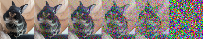
Most descriptions of diffusion models consider a process that gradually corrupts examples of a data distribution with noise. The task of the model is then to learn how to undo the corruption. Additive Gaussian noise is most commonly used as the corruption method. This has the nice property that adding noise multiple times in sequence yields the same outcome (in a distributional sense) as adding noise once with a higher standard deviation. The total standard deviation is found as \(\sigma = \sqrt{ \sum_i \sigma_i^2}\), where \(\sigma_1, \sigma_2, \ldots\) are the standard deviations of the noise added at each point in the sequence.

Therefore, at each point in the corruption process, we can ask: what is the total amount of noise that has been added so far – what is its standard deviation? We can write this as \(\sigma(t)\), where \(t\) is a time variable that indicates how far the corruption process has progressed. This function \(\sigma(t)\) is what we typically refer to as the noise schedule. Another consequence of this property of Gaussian noise is that we can jump forward to any point in the corruption process in a single step, simply by adding noise with standard deviation \(\sigma(t)\) to a noiseless input example. The distribution of the result is exactly the same as if we had run the corruption process step by step.

In addition to adding noise, the original noiseless input is often rescaled by a time-dependent scale factor \(\alpha(t)\) to stop it from growing uncontrollably. Given an example \(\mathbf{x}_0\), we can turn it into a noisy example \(\mathbf{x}_t = \alpha(t) \mathbf{x}_0 + \sigma(t) \varepsilon\), where \(\varepsilon \sim \mathcal{N}(0, 1)\).

• The most popular formulation of diffusion models chooses \(\alpha(t) = \sqrt{1 - \sigma(t)^2}\), which also requires that \(\sigma(t) \leq 1\). This is because if we assume \(\mathrm{Var}[\mathbf{x}_0] = 1\), we can derive that \(\mathrm{Var}[\mathbf{x}_t] = 1\) for all \(t\). In other words, this choice is variance-preserving: the total variance (of the signal plus the added noise) is \(1\) at every step of the corruption process. In the literature, this is referred to as VP diffusion¹. While \(\mathrm{Var}[\mathbf{x}_0] = 1\) isn’t always true in practice (for example, image pixels scaled to \([-1, 1]\) will have a lower variance), it’s often close enough that things still work well in practice.

• An alternative is to do no rescaling at all, i.e. \(\alpha(t) = 1\). This is called variance-exploding or VE diffusion. It requires \(\sigma(t)\) to grow quite large to be able to drown out all of the signal for large values of \(t\), which is a prerequisite for diffusion models to work well. For image pixels scaled to \([-1, 1]\), we might want to ramp up \(\sigma(t)\) all the way to ~100 before it becomes more or less impossible to discern any remaining signal structure. The exact maximum value is a hyperparameter which depends on the data distribution. It was popularised by Karras et al. (2022)².

• More recently, formalisms based on flow matching³ and rectified flow⁴ have gained popularity. They set \(\alpha(t) = 1 - \sigma(t)\), which is also sometimes referred to as sub-VP diffusion. This is because in this case, \(\mathrm{Var}[\mathbf{x}_t] \leq 1\) when we assume \(\mathrm{Var}[\mathbf{x}_0] = 1\). This choice is supposed to result in straighter paths through input space between data and noise, which in turn reduces the number of sampling steps required to hit a certain level of quality (see my previous blog post for more about sampling with fewer steps). Stable Diffusion 3 uses this approach⁵.

By convention, \(t\) typically ranges from \(0\) to \(1\) in the VP and sub-VP settings, so that no noise is present at \(t=0\) (hence \(\sigma(0) = 0\) and \(\alpha(t) = 1\)), and at \(t=1\) the noise has completely drowned out the signal (hence \(\sigma(1) = 1\) and \(\alpha(1) = 0\)). In the flow matching literature, the direction of \(t\) is usually reversed, so that \(t=0\) corresponds to maximal noise and \(t=1\) to minimal noise instead, but I am sticking to the diffusion convention here. Note that \(t\) can be a continuous time variable, or a discrete index, depending on which paper you’re reading; here, we will assume it is continuous.

Let’s look at a few different noise schedules that have been used in the literature. It goes without saying that this is far from an exhaustive list – I will only mention some of the most popular and interesting options.

• The so-called linear schedule was proposed in the original DDPM paper⁶. This paper uses a discrete-time formulation, and specifies the schedule in terms of the variances of \(q(\mathbf{x}_{t+1} \mid \mathbf{x}_t)\) (corresponding to a single discrete step in the forward process), which they call \(\beta_t\). These variances increase linearly with \(t\), which is where the name comes from. In our formalism, this corresponds to \(\sigma(t) = \sqrt{\sum_{i=1}^t \beta_i}\), so while \(\beta_t\) might be a linear function of \(t\), \(\sigma(t)\) is not.

• The cosine schedule is arguably the most popular noise schedule to this day. It was introduced by Nichol & Dhariwal⁷ after observing that the linear schedule is suboptimal for high-resolution images, because it gets too noisy too quickly. This corresponds to \(\sigma(t) = \sin \left(\frac{t/T + s}{1 + s} \frac{\pi}{2} \right)\), where \(T\) is the maximal (discrete) time step, and \(s\) is an offset hyperparameter. It might seem like calling this the sine schedule would have been more appropriate, but the naming is again the result of using a slightly different formalism. (There is no standardised formalism for diffusion models, so every paper tends to describe things using different conventions and terminology, which is something I’ve written about before.)

• Karras et al. (2022)² use the variance-exploding formalism in combination with the simplest noise schedule you can imagine: \(\sigma(t) = t\). Because of this, they get rid of the “time” variable altogether, and express everything directly in terms of \(\sigma\) (because they are effectively equivalent). This is not the whole story however, and we’ll revisit this approach later.

• To adjust a pre-existing noise schedule to be more suitable for high-resolution images, both Chen (2023)⁸ and Hoogeboom et al. (2023)⁹ suggest “shifting” the schedule to account for the fact that neighbouring pixels in high-resolution images exhibit much stronger correlations than in low-resolution images, so more noise is needed to obscure any structure that is present. They do this by expressing the schedule in terms of the signal-to-noise ratio, \(\mathrm{SNR}(t) = \frac{\alpha(t)^2}{\sigma(t)^2}\), and showing that halving the resolution along both the width and height dimensions (dividing the total number of pixels by 4) requires scaling \(SNR(t)\) by a factor of 4 to ensure the same level of corruption at time \(t\). If we express the noise schedule in terms of the logarithm of the SNR, this means we simply have to additively shift the input by \(\log 4\), or by \(- \log 4\) when doubling the resolution instead.

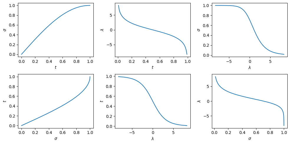
There is a monotonically decreasing (and hence, invertible) relationship between the time variable of the diffusion process and the logSNR. Representing things in terms of the logSNR instead of time is quite useful: it is a direct measure of the amount of information obscured by noise, and is therefore easier to compare across different settings: different models, different noise schedules, but also across VP, VE and sub-VP formulations.

Noise levels: focusing on what matters

Let’s dive a bit deeper into the role that noise schedules fulfill. Compared to other classes of generative models, diffusion models have a superpower: because they generate things step-by-step in a coarse-to-fine or hierarchical manner, we can determine which levels of this hierarchy are most important to us, and use the bulk of their capacity for those. There is a very close correspondence between noise levels and levels of the hierarchy.

This enables diffusion models to be quite compute- and parameter-efficient for perceptual modalities in particular: sound, images and video exhibit a huge amount of variation in relative importance across different levels of granularity, with respect to perceptual quality. More concretely, human eyes and ears are much more sensitive to low frequencies than high frequencies, and diffusion models can exploit this out of the box by spending more effort on modelling lower frequencies, which correspond to higher noise levels. (Incidentally, I believe this is one of the reasons why they haven’t really caught on for language modelling, where this advantage does not apply – I have a blog post about that as well.)

In what follows, I will focus on these perceptual use cases, but the observations and conclusions are also applicable to diffusion models of other modalities. It’s just convenient to talk about perceptual quality as a stand-in for “aspects of sample quality that we care about”.

So which noise levels should we focus on when training a diffusion model, and how much? I believe the two most important matters that affect this decision are:

• the perceptual relevance of each noise level, as previously discussed;
• the difficulty of the learning task at each noise level.

Neither of these are typically uniformly distributed. It’s also important to consider that these distributions are not necessarily similar to each other: a noise level that is highly relevant perceptually could be quite easy for the model to learn to make predictions for, and vice versa. Noise levels that are particularly difficult could be worth focusing on to improve output quality, but they could also be so difficult as to be impossible to learn, in which case any effort expended on them would be wasted.

To find the optimal balance between noise levels during model training, we need to take both perceptual relevance and difficulty into account. This always comes down to a trade-off between different priorities: model capacity is finite, and focusing training on certain noise levels will necessarily reduce a model’s predictive capability at other noise levels.

When sampling from a trained diffusion model, the situation is a bit different. Here, we need to choose how to space things out as we traverse the different noise levels from high to low. In a range of noise levels that is more important, we’ll want to spend more time evaluating the model, and therefore space the noise levels closer together. As the number of sampling steps we can afford is usually limited, this means we will have to space the noise levels farther apart elsewhere. The importance of noise levels during sampling is affected by:

• their perceptual relevance, as is the case for model training;
• the accuracy of model predictions;
• the possibility for accumulation of errors.

While prediction accuracy is of course closely linked to the difficulty of the learning task, it is not the same thing. The accumulation of errors over the course of the sampling process also introduces an asymmetry, as errors made early in the process (at high noise levels) are more likely to lead to problems than those made later on (at low noise levels). These subtle differences can result in an optimal balance between noise levels that looks very different than at training time, as we will see later.

Model design choices: what might tip the balance?

Now that we have an idea of what affects the relative importance of noise levels, both for training and sampling, we can analyse the various design choices we need to make when constructing a diffusion model, and how they influence this balance. As it turns out, the choice of noise schedule is far from the only thing that matters.

A good starting point is to look at how we estimate the training loss:

Here, \(p(\mathbf{x}_0)\) is the data distribution, and \(p(\mathbf{x}_t \mid \mathbf{x}_0, t)\) represents the so-called transition density of the forward diffusion process, which describes the distribution of the noisy input \(\mathbf{x}_t\) at time step \(t\) if we started the corruption process at a particular training example \(\mathbf{x}_0\) at \(t = 0\). In addition to the noise schedule \(\sigma(t)\), there are three aspects of the loss that together determine the relative importance of noise levels: the model output parameterisation \(\color{purple}{f(\mathbf{x}_t, t)}\), the loss weighting \(\color{blue}{w(t)}\) and the time step distribution \(\color{red}{p(t)}\). We’ll take a look at each of these in turn.

Model output parameterisation \(\color{purple}{f(\mathbf{x}_t, t)}\)

For a typical diffusion model, we sample from the transition density in practice by sampling standard Gaussian noise \(\varepsilon \sim \mathcal{N}(0, 1)\) and constructing \(\mathbf{x}_t = \alpha(t) \mathbf{x}_0 + \sigma(t) \varepsilon\), i.e. a weighted mix of the data distribution and standard Gaussian noise, with \(\sigma(t)\) the noise schedule and \(\alpha(t)\) defined accordingly (see Section 1). This implies that the transition density is Gaussian: \(p(\mathbf{x}_t \mid \mathbf{x}_0, t) = \mathcal{N}(\alpha(t) \mathbf{x}_0, \sigma(t)^2)\).

Here, we have chosen to parameterise the model \(\color{purple}{f(\mathbf{x}_t, t)}\) to predict the corresponding clean input \(\mathbf{x}_0\), following Karras et al.². This is not the only option: it is also common to have the model predict \(\varepsilon\), or a linear combination of the two, which can be time-dependent (as in \(\mathbf{v}\)-prediction¹⁰, \(\mathbf{v} = \alpha(t) \varepsilon - \sigma(t) \mathbf{x}_0\), or as in rectified flow⁴, where the target is \(\varepsilon - \mathbf{x}_0\)).

Once we have a prediction \(\hat{\mathbf{x}}_0 = \color{purple}{f(\mathbf{x}_t, t)}\), we can easily turn this into a prediction \(\hat{\varepsilon}\) or \(\hat{\mathbf{v}}\) corresponding to a different parameterisation, using the linear relation \(\mathbf{x}_t = \alpha(t) \mathbf{x}_0 + \sigma(t) \varepsilon\), because \(t\) and \(\mathbf{x}_t\) are given. You would be forgiven for thinking that this implies all of these parameterisations are essentially equivalent, but that is not the case.

Depending on the choice of parameterisation, different noise levels will be emphasised or de-emphasised in the loss, which is an expectation across all time steps. To see why, consider the expression \(\mathbb{E}[(\hat{\mathbf{x}_0} - \mathbf{x}_0)^2]\), i.e. the mean squared error w.r.t. the clean input \(\mathbf{x}_0\), which we can rewrite in terms of \(\varepsilon\):

The factor \(\frac{\sigma(t)^2}{\alpha(t)^2}\) which appears in front is the reciprocal of the signal-to-noise ratio \(\mathrm{SNR}(t) = \frac{\alpha(t)^2}{\sigma(t)^2}\). As a result, when we switch our model output parameterisation from predicting \(\mathbf{x}_0\) to predicting \(\varepsilon\) instead, we are implicitly introducing a relative weighting factor equal to \(\mathrm{SNR}(t)\).

We can also rewrite the MSE in terms of \(\mathbf{v}\):

In the VP case, the denominator is equal to \(1\).

These implicit weighting factors will compound with other design choices to determine the relative contribution of each noise level to the overall loss, and therefore, influence the way model capacity is distributed across noise levels. Concretely, this means that a noise schedule tuned to work well for a model that is parameterised to predict \(\mathbf{x}_0\), cannot be expected to work equally well when we parameterise the model to predict \(\varepsilon\) or \(\mathbf{v}\) instead (or vice versa).

This is further complicated by the fact that the model output parameterisation also affects the feasibility of the learning task at different noise levels: predicting \(\varepsilon\) at low noise levels is more or less impossible, so the optimal thing to do is to predict the mean (which is 0). Conversely, predicting \(\mathbf{x}_0\) is challenging at high noise levels, although somewhat more constrained in the conditional setting, where the optimum is to predict the conditional mean across the dataset.

Aside: to disentangle these two effects, one could parameterise the model to predict one quantity (e.g. \(\mathbf{x}_0\)), convert the model predictions to another parameterisation (e.g. \(\varepsilon\)), and express the loss in terms of that, thus changing the implicit weighting. However, this can also be achieved simply by changing \(\color{blue}{w(t)}\) or \(\color{red}{p(t)}\) instead.

Loss weighting \(\color{blue}{w(t)}\)

Many diffusion model formulations feature an explicit time-dependent weighting function in the loss. Karras et al.²’s formulation (often referred to as EDM) features an explicit weighting function \(\lambda(\sigma)\), to compensate for the implicit weighting induced by their choice of parameterisation.

In the original DDPM paper⁶, this weighting function arises from the derivation of the variational bound, but is then dropped to obtain the “simple” loss function in terms of \(\varepsilon\) (§3.4 in the paper). This is found to improve sample quality, in addition to simplifying the implementation. Dropping the weighting results in low noise levels being downweighted considerably compared to high ones, relative to the variational bound. For some applications, keeping this weighting is useful, as it enables training of diffusion models to maximise the likelihood in the input space^{11 12} – lossless compression is one such example.

Time step distribution \(\color{red}{p(t)}\)

During training, a random time step is sampled for each training example \(\mathbf{x}_0\). Most formulations sample time steps uniformly (including DDPM), but some, like EDM² and Stable Diffusion 3⁵, choose a different distribution instead. It stands to reason that this will also affect the balance between noise levels, as some levels will see a lot more training examples than others.

Note that a uniform distribution of time steps usually corresponds to a non-uniform distribution of noise levels, because \(\sigma(t)\) is a nonlinear function. In fact, in the VP case (where \(t, \sigma \in [0, 1]\)), it is precisely the inverse of the cumulative distribution function (CDF) of the resulting noise level distribution.

It turns out that \(\color{blue}{w(t)}\) and \(\color{red}{p(t)}\) are in a sense interchangeable. To see this, simply write out the expectation over \(t\) in the loss as an integral:

It’s pretty obvious now that we are really just multiplying the density of the time step distribution \(\color{red}{p(t)}\) with the weighting function \(\color{blue}{w(t)}\), so we could just absorb \(\color{red}{p(t)}\) into \(\color{blue}{w(t)}\) and make the time step distribution uniform:

Alternatively, we could absorb \(\color{blue}{w(t)}\) into \(\color{red}{p(t)}\) instead. We may have to renormalise it to make sure it is still a valid distribution, but that’s okay, because scaling a loss function by an arbitrary constant factor does not change where the minimum is:

So why would we want to use \(\color{blue}{w(t)}\) or \(\color{red}{p(t)}\), or some combination of both? In practice, we train diffusion models with minibatch gradient descent, which means we stochastically estimate the expectation through sampling across batches of data. The integral over \(t\) is estimated by sampling a different value for each training example. In this setting, the choice of \(\color{red}{p(t)}\) and \(\color{blue}{w(t)}\) affects the variance of said estimate, as well as that of its gradient. For efficient training, we of course want the loss estimate to have the lowest variance possible, and we can use this to inform our choice¹¹.

You may have recognised this as the key idea behind importance sampling, because that’s exactly what this is.

Time step spacing

Once a model is trained and we want to sample from it, \(\color{blue}{w(t)}\), \(\color{red}{p(t)}\) and the choice of model output parameterisation are no longer of any concern. The only thing that determines the relative importance of noise levels at this point, apart from the noise schedule \(\sigma(t)\), is how we space the time steps at which we evaluate the model in order to produce samples.

In most cases, time steps are uniformly spaced (think np.linspace) and not much consideration is given to this. Note that this spacing of time steps usually gives rise to a non-uniform spacing of noise levels, because the noise schedule \(\sigma(t)\) is typically nonlinear.

An exception is EDM², with its simple (linear) noise schedule \(\sigma(t) = t\). Here, the step spacing is intentionally done in a nonlinear fashion, to put more emphasis on lower noise levels. Another exception is the DPM-Solver paper¹³, where the authors found that their proposed fast deterministic sampling algorithm benefits from uniform spacing of noise levels when expressed in terms of logSNR. The latter example demonstrates that the optimal time step spacing can also depend on the choice of sampling algorithm. Stochastic algorithms tend to have better error-correcting properties than deterministic ones, reducing the potential for errors to accumulate over multiple steps².

Noise schedules are a superfluous abstraction

With everything we’ve discussed in the previous two sections, you might ask: what do we actually need the noise schedule for? What role does the “time” variable \(t\) play, when what we really care about is the relative importance of noise levels?

Good question! We can reexpress the loss from the previous section directly in terms of the standard deviation of the noise \(\sigma\):

This is actually quite a straightforward change of variables, because \(\sigma(t)\) is a monotonic and invertible function of \(t\). I’ve also gone ahead and replaced the subscripts \(t\) with \(\sigma\) instead. Note that this is a slight abuse of notation: \(\color{blue}{w(\sigma)}\) and \(\color{blue}{w(t)}\) are not the same functions applied to different arguments, they are actually different functions. The same holds for \(\color{red}{p}\) and \(\color{purple}{f}\). (Adding additional subscripts or other notation to make this difference explicit seemed like a worse option.)

Another possibility is to express everything in terms of the logSNR \(\lambda\):

This is again possible because of the monotonic relationship that exists between \(\lambda\) and \(t\) (and \(\sigma\), for that matter). One thing to watch out for when doing this, is that high logSNRs \(\lambda\) correspond to low standard deviations \(\sigma\), and vice versa.

Once we perform one of these substitutions, the time variable becomes superfluous. This shows that the noise schedule does not actually add any expressivity to our formulation – it is merely an arbitrary nonlinear function that we use to convert back and forth between the domain of time steps and the domain of noise levels. In my opinion, that means we are actually making things more complicated than they need to be.

I’m hardly the first to make this observation: Karras et al. (2022)² figured this out about two years ago, which is why they chose \(\sigma(t) = t\), and then proceeded to eliminate \(t\) everywhere, in favour of \(\sigma\). One might think this is only possible thanks to the variance-exploding formulation they chose to use, but in VP or sub-VP formulations, one can similarly choose to express everything in terms of \(\sigma\) or \(\lambda\) instead.

In addition to complicating things with a superfluous variable and unnecessary nonlinear functions, I have a few other gripes with noise schedules:

• They needlessly entangle the training and sampling importance of noise levels, because changing the noise schedule simultaneously impacts both. This leads to people doing things like using different noise schedules for training and sampling, when it makes more sense to modify the training weighting and sampling spacing of noise levels directly.

• They cause confusion: a lot of people are under the false impression that the noise schedule (and only the noise schedule) is what determines the relative importance of noise levels. I can’t blame them for this misunderstanding, because it definitely sounds plausible based on the name, but I hope it is clear at this point that this is not accurate.

• When combining a noise schedule with uniform time step sampling and uniform time step spacing, as is often done, there is an underlying assumption that specific noise levels are equally important for both training and sampling. This is typically not the case (see Section 2), and the EDM paper also supports this by separately tuning the noise level distribution \(\color{red}{p(\sigma)}\) and the sampling spacing. Kingma & Gao¹⁴ express these choices as weighting functions in terms of the logSNR, demonstrating just how different they end up being (see Figure 2 in their paper).

So do noise schedules really have no role to play in diffusion models? That’s probably an exaggeration. Perhaps they were a necessary concept that had to be invented to get to where we are today. They are pretty key in connecting diffusion models to the theory of stochastic differential equations (SDEs) for example, and seem inevitable in any discrete-time formalism. But for practitioners, I think the concept does more to muddy the waters than to enhance our understanding of what’s going on. Focusing instead on noise levels and their relative importance allows us to tease apart the differences between training and sampling, and to design our models to have precisely the weighting we intended.

This also enables us to cast various formulations of diffusion and diffusion-adjacent models (e.g. flow matching³ / rectified flow⁴, inversion by direct iteration¹⁵, …) as variants of the same idea with different choices of noise level weighting, spacing and scaling. I strongly recommend taking a look at appendix D of Kingma & Gao’s “Understanding diffusion objectives” paper for a great overview of these relationships. In Section 2 and Appendix C of the EDM paper, Karras et al. perform a similar exercise, and this is also well worth reading. The former expresses everything in terms of the logSNR \(\lambda\), the latter uses the standard deviation \(\sigma\).

Adaptive weighting mechanisms

A few heuristics and mechanisms to automatically balance the importance of different noise levels have been proposed in the literature, both for training and sampling. I think this is a worthwhile pursuit, because optimising what is essentially a function-valued hyperparameter can be quite costly and challenging in practice. For some reason, these ideas are frequently tucked away in the appendices of papers that make other important contributions as well.

• The “Variational Diffusion Models” paper¹¹ uses a fixed noise level weighting for training, corresponding to the likelihood loss (or rather, a variational bound on it). But as we discussed earlier, given a particular choice of model output parameterisation, any weighting can be implemented either through an explicit weighting factor \(\color{blue}{w(t)}\), a non-uniform time step distribution \(\color{red}{p(t)}\), or some combination of both, which affects the variance of the loss estimate. They show how this variance can be minimised explicitly by parameterising the noise schedule with a neural network, and optimising its parameters to minimise the squared diffusion loss, alongside the denoising model itself (see Appendix I.2). This idea is also compatible with other choices of noise level weighting.

• The “Understanding Diffusion Objectives” paper¹⁴ proposes an alternative online mechanism to reduce variance. Rather than minimising the variance directly, expected loss magnitude estimates are tracked across a range of logSNRs divided into a number of discrete bins, by updating an exponential moving average (EMA) after every training step. These are used for importance sampling: we can construct an adaptive piecewise constant non-uniform noise level distribution \(\color{red}{p(\lambda)}\) that is proportional to these estimates, which means noise levels with a higher expected loss value will be sampled more frequently. This is compensated for by multiplying the explicit weighting function \(\color{blue}{w(\lambda)}\) by the reciprocal of \(\color{red}{p(\lambda)}\), which means the effective weighting is kept unchanged (see Appendix F).

• In “Analyzing and Improving the Training Dynamics of Diffusion Models”, also known as the EDM2 paper¹⁶, Karras et al. describe another adaptation mechanism which at first glance seems quite similar to the one above, because it also works by estimating loss magnitudes (see Appendix B.2). There are a few subtle but crucial differences, though. Their aim is to keep gradient magnitudes across different noise levels balanced throughout training. This is achieved by adapting the explicit weighting \(\color{blue}{w(\sigma)}\) over the course of training, instead of modifying the noise level distribution \(\color{red}{p(\sigma)}\) as in the preceding method (here, this is kept fixed throughout). The adaptation mechanism is based on a multi-task learning approach¹⁷, which works by estimating the loss magnitudes across noise levels with a one-layer MLP, and normalising the loss contributions accordingly. The most important difference is that this is not compensated for by adapting \(\color{red}{p(\sigma)}\), so this mechanism actually changes the effective weighting of noise levels over the course of training, unlike the previous two.

• In “Continuous diffusion for categorical data” (CDCD), my colleagues and I developed an adaptive mechanism we called “time warping”¹⁸. We used the categorical cross-entropy loss to train diffusion language models – the same loss that is also used to train autoregressive language models. Time warping tracks the cross-entropy loss values across noise levels using a learnable piecewise linear function. Rather than using this information for adaptive rescaling, the learnt function is interpreted as the (unnormalised) cumulative distribution function (CDF) of \(\color{red}{p(\sigma)}\). Because the estimate is piecewise linear, we can easily normalise it and invert it, enabling us to sample from \(\color{red}{p(\sigma)}\) using inverse transform sampling (\(\color{blue}{w(\sigma)} = 1\) is kept fixed). If we interpret the cross-entropy loss as measuring the uncertainty of the model in bits, the effect of this procedure is to balance model capacity between all bits of information contained in the data.

• In “Continuous Diffusion for Mixed-Type Tabular Data”, Mueller et al.¹⁹ extend the time warping mechanism to heterogeneous data, and use it to learn different noise level distributions \(\color{red}{p(\sigma)}\) for different data types. This is useful in the context of continuous diffusion on embeddings which represent discrete categories, because a given corruption process may destroy the underlying categorical information at different rates for different data types. Adapting \(\color{red}{p(\sigma)}\) to the data type compensates for this, and ensures information is destroyed at the same rate across all data types.

All of the above mechanisms adapt the noise level weighting in some sense, but they vary along a few axes:

• Different aims: minimising the variance of the loss estimate, balancing the magnitude of the gradients, balancing model capacity, balancing corruption rates across heterogeneous data types.
• Different tracking methods: EMA, MLPs, piecewise linear functions.
• Different ways of estimating noise level importance: squared diffusion loss, measuring the loss magnitude directly, multi-task learning, fitting the CDF of \(\color{red}{p(\sigma)}\).
• Different ways of employing this information: it can be used to adapt \(\color{red}{p}\) and \(\color{blue}{w}\) together, only \(\color{red}{p}\), or only \(\color{blue}{w}\). Some mechanisms change the effective weighting \(\color{red}{p} \cdot \color{blue}{w}\) over the course of training, others keep it fixed.

Apart from these online mechanisms, which adapt hyperparameters on-the-fly over the course of training, one can also use heuristics to derive weightings offline that are optimal in some sense. Santos & Lin (2023) explore this setting, and propose four different heuristics to obtain noise schedules for continuous variance-preserving Gaussian diffusion²⁰. One of them, based on the Fisher Information, ends up recovering the cosine schedule. This is a surprising result, given its fairly ad-hoc origins. Whether there is a deeper connection here remains to be seen, as this derivation does not account for the impact of perceptual relevance on the relative importance of noise levels, which I think plays an important role in the success of the cosine schedule.

The mechanisms discussed so far apply to model training. We can also try to automate finding the optimal sampling step spacing for a trained model. A recent paper titled “Align your steps”²¹ proposes to optimise the spacing by analytically minimising the discretisation error that results from having to use finite step sizes. For smaller step budgets, some works have treated the individual time steps as sampling hyperparameters that can be optimised via parameter sweeping or black-box optimisation: the WaveGrad paper²² is an example where a high-performing schedule with only 6 steps was found in this way.

In CDCD, we found that reusing the learnt CDF of \(\color{red}{p(\sigma)}\) to also determine the sampling spacing of noise levels worked very well in practice. This seemingly runs counter to the observation made in the EDM paper², that optimising the sampling spacing separately from the training weighting is worthwhile. My current hypothesis for this is as follows: in the language domain, information is already significantly compressed, to such an extent that every bit ends up being roughly equally important for output quality and performance on downstream tasks. (This also explains why balancing model capacity across all bits during training works so well in this setting.) We know that this is not the case at all for perceptual signals such as images: for every perceptually meaningful bit of information in an uncompressed image, there are 99 others that are pretty much irrelevant (which is why lossy compression algorithms such as JPEG are so effective).

Closing thoughts

I hope I have managed to explain why I am not a huge fan of the noise schedule as a central abstraction in diffusion model formalisms. The balance between different noise levels is determined by much more than just the noise schedule: the model output parameterisation, the explicit time-dependent weighting function (if any), and the distribution which time steps are sampled from all have a significant impact during training. When sampling, the spacing of time steps also plays an important role.

All of these should be chosen in tandem to obtain the desired relative weighting of noise levels, which might well be different for training and sampling, because the optimal weighting in each setting is affected by different things: the difficulty of the learning task at each noise level (training), the accuracy of model predictions (sampling), the possibility for error accumulation (sampling) and the perceptual relevance of each noise level (both). An interesting implication of this is that finding the optimal weightings for both settings actually requires bilevel optimisation, with an outer loop optimising the training weighting, and an inner loop optimising the sampling weighting.

As a practitioner, it is worth being aware of how all these things interact, so that changing e.g. the model output parameterisation does not lead to a surprise drop in performance, because the accompanying implicit change in the relative weighting of noise levels was not accounted for. The “noise schedule” concept unfortunately creates the false impression that it solely determines the relative importance of noise levels, and needlessly entangles them across training and sampling. Nevertheless, it is important to understand the role of noise schedules, as they are pervasive in the diffusion literature.

Two papers were instrumental in developing my own understanding: the EDM paper² (yes, I am aware that I’m starting to sound like a broken record!) and the “Understanding diffusion objectives” paper¹⁴. They are both really great reads (including the various appendices), and stuffed to the brim with invaluable wisdom. In addition, the recent Stable Diffusion 3 paper⁵ features a thorough comparison study of different noise schedules and model output parameterisations.

I promised I would explain the title: this is of course a reference to Dijkstra’s famous essay about the “go to” statement. It is perhaps the most overused of all snowclones in technical writing, but I chose it specifically because the original essay also criticised an abstraction that sometimes does more harm than good.

This blog post took a few months to finish, including several rewrites, because the story is quite nuanced. The precise points I wanted to make didn’t become clear even to myself, until about halfway through writing it, and my thinking on this issue is still evolving. If anything is unclear (or wrong!), please let me know. I am curious to learn if there are any situations where an explicit time variable and/or a noise schedule simplifies or clarifies things, which would not be obvious when expressed directly in terms of the standard deviation \(\sigma\), or the logSNR \(\lambda\). I also want to know about any other adaptive mechanisms that have been tried. Let me know in the comments, or come find me at ICML 2024 in Vienna!

If you would like to cite this post in an academic context, you can use this BibTeX snippet:

@misc{dieleman2024schedules,
  author = {Dieleman, Sander},
  title = {Noise schedules considered harmful},
  url = {https://sander.ai/2024/06/14/noise-schedules.html},
  year = {2024}
}

Acknowledgements

Thanks to Robin Strudel, Edouard Leurent, Sebastian Flennerhag and all my colleagues at Google DeepMind for various discussions, which continue to shape my thoughts on diffusion models and beyond!

References