Ever since the rise of diffusion models, people have sought ways to make them faster and cheaper to sample from. About two years ago, I wrote a blog post about diffusion distillation, which is one of the main tools used to reduce the number of steps required to obtain high-quality samples. Although the core principles underlying various distillation methods have not changed, a lot of new variants have popped up since.

In this blog post, I want to take a closer look at flow maps. While diffusion models describe paths between noise and data by predicting the tangent direction at each point along the path, flow maps are instead able to predict any point on a path from any other point on that same path. They can be used for faster sampling, but they also have some other tricks up their sleeve, enabling more efficient reward-based learning and improved sampling steerability, among other things. They have recently become a very popular subject of study.

While it is relatively straightforward to define what a flow map is, there turn out to be many different ways to build and train them. On top of that, as with diffusion itself, the literature is once again rife with different formalisms and terminology, which makes for a confusing experience when trying to learn how everything fits together. I will do my best to clear things up a bit, based primarily on the taxonomy proposed by Boffi et al.^{1 2}.

Flow maps build on the ideas behind diffusion models, and as usual, I will assume some familiarity with these ideas. Being comfortable with vector calculus will also help to understand how they are trained, but if that’s not you, hopefully the other parts of this blog post will still be interesting to you. You may want to consider (re-)reading some of my earlier blog posts for context (e.g. Perspectives on diffusion). Alternatively, Chieh-Hsin Lai and colleagues recently published a comprehensive monograph on diffusion models³, which combines math and rigour with intuitive explanations – highly recommended, both as a refresher and as a starting point.

Below is a table of contents. Click to jump directly to a particular section of this post.

1. Charting paths from noise to data
2. Three notions of consistency
3. To backprop or not to backprop?
4. Training flow maps from scratch
5. Flow maps in practice
6. Applications and extensions
7. Alternative strategies
8. Closing thoughts
9. Acknowledgements
10. References

Charting paths from noise to data

The key to understanding flow maps is the perspective of diffusion models as defining a bijection between noise and data, with unique paths connecting pairs of samples from each distribution, in such a way that they never cross each other. Therefore, let’s first take a closer look at diffusion sampling algorithms, and build towards flow maps from there.

Sampling from diffusion models

There are many different sampling algorithms available for diffusion models nowadays, but they all fall into one of two categories: stochastic or deterministic. The miracle of deterministic sampling is something I have written about before, but it is worth recapping here, as it is fundamental to the development of flow maps.

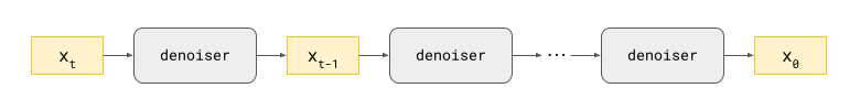
The gist of it is as follows: if we have a denoiser model that predicts the expected value of the clean original data \(\hat{\mathbf{x}}_0 = \mathbb{E}\left[ \mathbf{x}_0 \mid \mathbf{x}_t \right]\), given a noisy observation \(\mathbf{x}_t\), we can construct two distinct iterative generative procedures.

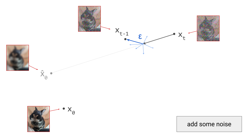
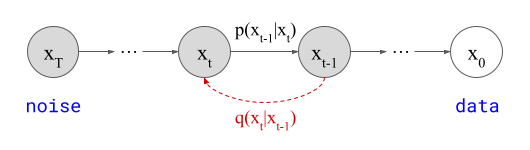
The stochastic one is the most intuitive: at each iteration, we sample from a conditional distribution of slightly less noisy examples, given the current noisy observation, \(p(\mathbf{x}_{t-1} \mid \mathbf{x}_t)\), to reverse the corruption process one step at a time. Conveniently, we can construct an approximation of this distribution using the denoiser model prediction \(\hat{\mathbf{x}}_0\). The smaller the interval between the noise levels at time steps \(t\) and \(t-1\), the more accurate the approximation will be. After many iterations, the noise fades, and we end up with a sample from the clean data distribution at \(t=0\). This is, in a nutshell, how the original DDPM⁴ algorithm works. Sampling algorithms based on the stochastic differential equation (SDE) formalism of diffusion models⁵ produce similar stochastic trajectories in input space.

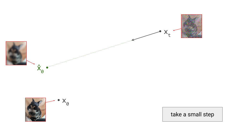
The deterministic procedure does not involve drawing random samples at any point, except at the very start: given the current noisy observation \(\mathbf{x}_t\) and the prediction \(\hat{\mathbf{x}}_0\) from the denoiser, there is a deterministic update rule that gives us \(\mathbf{x}_{t-1}\), which we can recursively apply until we get to \(\mathbf{x}_0\). Because every step of the procedure is deterministic, there is no randomness anywhere: from a given starting point \(\mathbf{x}_t\), we can only ever end up in one specific end point \(\mathbf{x}_0\). Such an update rule can be derived in the probabilistic framework (i.e. DDIM⁶), or using the ordinary differential equation (ODE) formalism⁵.

The default sampling algorithm used in Flow Matching⁷ is another instance of the deterministic procedure. Here, the neural network is typically parameterised to predict the velocity \(\mathbf{v}_t = \mathbb{E}\left[\mathbf{x}_T - \mathbf{x}_0 \mid \mathbf{x}_t \right]\) instead of the clean input \(\mathbb{E}\left[ \mathbf{x}_0 \mid \mathbf{x}_t \right]\) (with \(t=T\) the time step corresponding to the maximal noise level, i.e. pure Gaussian noise). However, as there is a linear relationship between \(\mathbf{v}_t\), \(\hat{\mathbf{x}}_0\) and \(\mathbf{x}_t\), this just yields a variant of the same underlying algorithm (see also this discussion of different diffusion model output parameterisations in an earlier blog post).

All these algorithms have in common that the marginal distributions of noisy examples \(p(\mathbf{x}_t)\) at each time step \(t\) are preserved: the distribution of \(\mathbf{x}_t\) does not depend on whether you chose to use a deterministic or stochastic sampling algorithm! This is of course not true at all for the conditional distributions \(p(\mathbf{x}_t \mid \mathbf{x}_T)\), which collapse to delta distributions in the deterministic case (all probability mass is on a single option). This preservation of the marginal distributions is also true for the special cases \(p(\mathbf{x}_0)\) and \(p(\mathbf{x}_T)\), at the data and noise sides respectively. If we look at specific individual examples rather than distributions, however, the path in input space traced out by the sampling process will look quite different.

Below is a visualisation of the sampling process: stochastic on the left, deterministic on the right. I decided to show this for both a 1D example (top) and a 2D example (bottom), because I believe the insights they provide are complementary. In both cases, the target distribution is a mixture of two Gaussians. We start with samples from our noise distribution, which is a single Gaussian. As sampling progresses, the distribution gradually transforms into the target mixture. The path a single sample traverses is quite jagged and erratic in the stochastic case, but smooth and gently curved in the deterministic case. Two very different microscopic behaviours give rise to the exact same macroscopic behaviour!

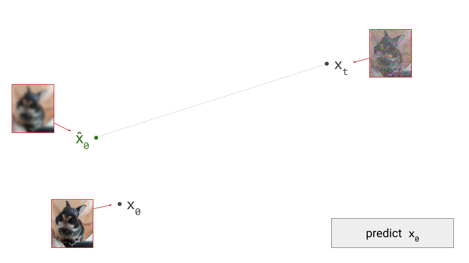
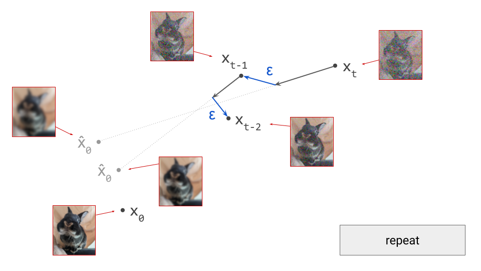
Dead reckoning: tracking paths with a diffusion model

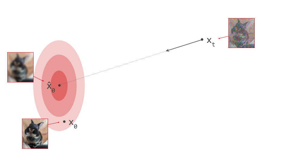
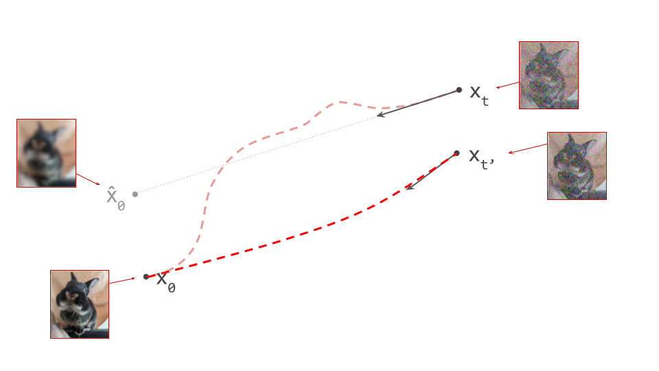
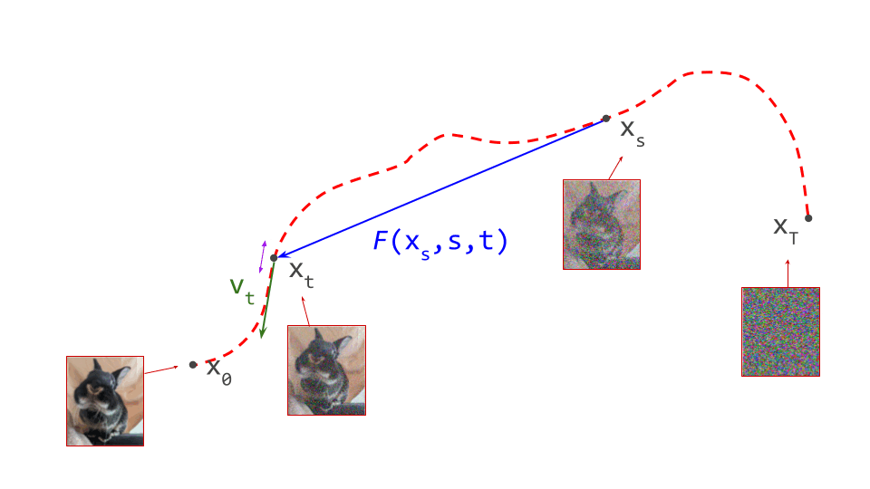
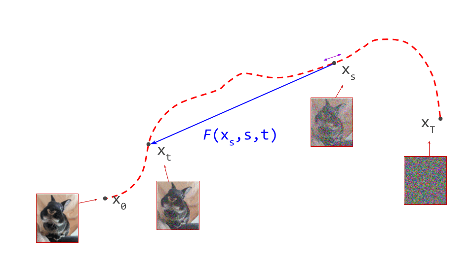
An important implication of the existence of deterministic sampling algorithms is that there must be a deterministic bijective mapping between individual samples from the noise and data distributions. Each noise sample is associated with a single specific data sample, and vice versa. Starting from a noise sample, we can follow a path through input space that leads us to the corresponding data sample. We do this simply by following the tangent direction to the path at each point, which is predicted by the denoiser. Note that we can also use the same tangent direction to guide us along the path in reverse, from data to noise.

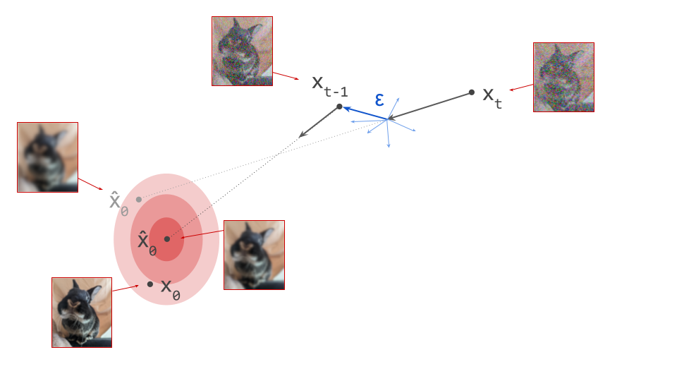
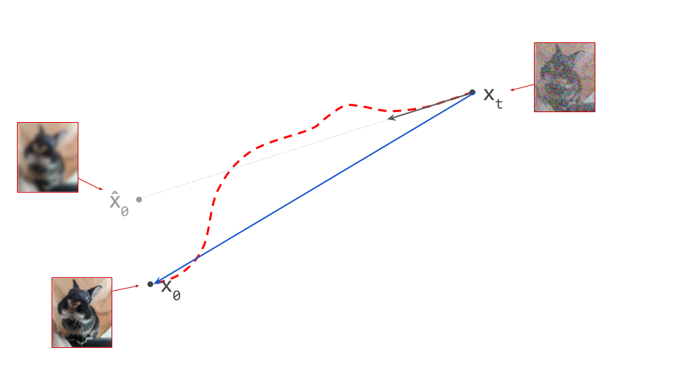
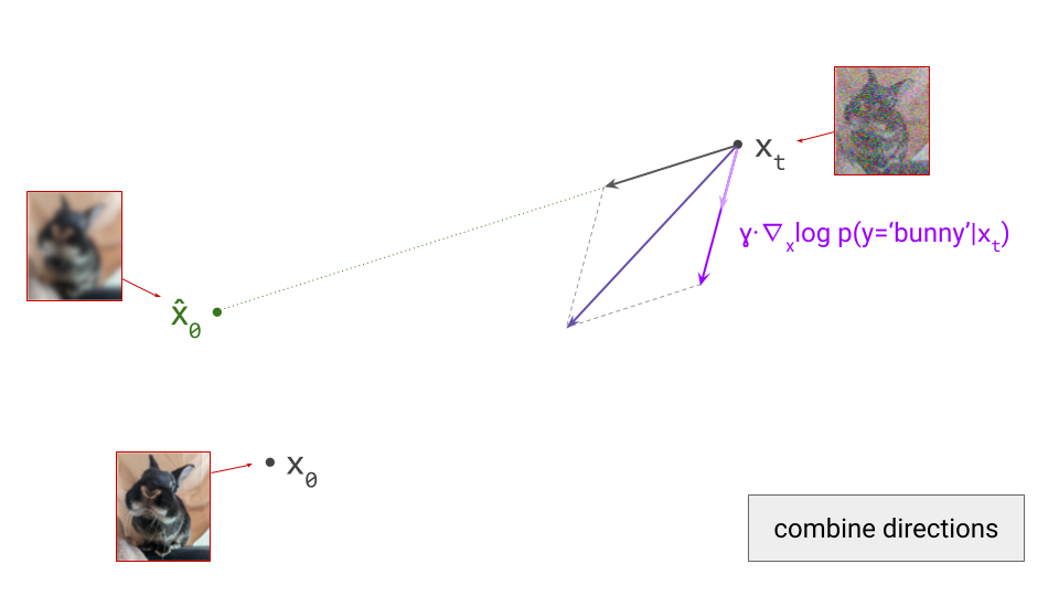
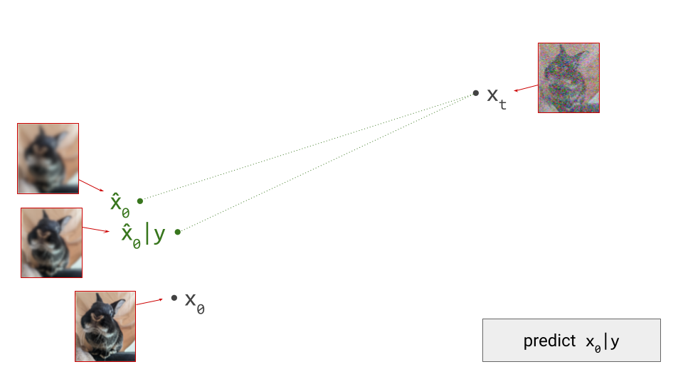
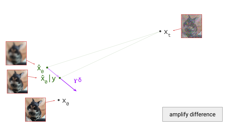
The diagram below shows a sample from the noise distribution \(\mathbf{x}_T\), the corresponding data sample \(\mathbf{x}_0\), the path through input space connecting them, and an intermediate point on the path \(\mathbf{x}_t\). It also shows the denoiser prediction \(\hat{\mathbf{x}}_0\) at this point, which corresponds to the tangent direction to the path. If you’ve read my previous posts on the geometry of guidance or distillation, you will probably be familiar with this type of diagram. The former post also contains a warning about the dangers of representing high-dimensional objects in 2D, which bears repeating: great care should be taken when drawing conclusions from 2D intuitions!

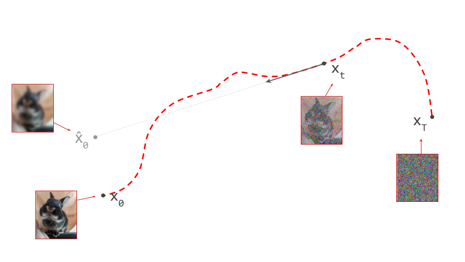
Using denoiser predictions to traverse these paths is memoryless: the only inputs to the denoiser are the current position in input space and the current noise level, from which it predicts a direction to move in, \(\hat{\mathbf{x}}_0 = f(\mathbf{x}_t, t)\). It is also myopic: the denoiser doesn’t get to peek ahead at the eventual destination \(\mathbf{x}_0\), it just says where to go next. It is not able to use any other information: no previously visited positions or previously predicted directions, no start- or endpoints, just where we are currently in the sampling process, and nothing else. This way of characterising paths brings to mind navigation through dead reckoning.

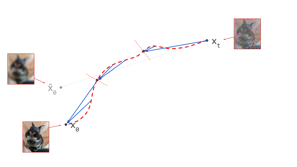
It follows that the path between a specific pair of noise and data samples that are connected in this way must be unique: if there were more than one path leading to a particular data sample, there would be multiple valid tangent directions at the point where these paths separate from each other. For the same reason, paths between different pairs of samples can never cross each other, because that would introduce ambiguity at the crossing point. It is not possible for the denoiser to distinguish between multiple crossing paths, because it only knows its current position, not which path it is on. This is shown in the diagram below.

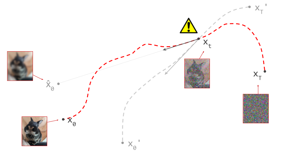
Technically, this argument only demonstrates that paths cannot cross in \((\mathbf{x}_t, t)\)-space, but they could still cross in \(\mathbf{x}_t\)-space in theory, if the two paths in question arrive at the same point in input space at different time steps \(t\). In practice, we can ignore this edge case, because the distributions of noisy intermediate samples \(p(\mathbf{x}_t)\) for two sufficiently different time steps will have basically no overlap. In fact, some recent papers^{8 9} suggest that not feeding the current noise level into the denoiser often works just as well or even better, because in a high-dimensional input space, it is able to infer the noise level from \(\mathbf{x}_t\) itself.

The fact that paths never cross in practice is what enables memoryless traversal using a denoiser. Paths are sometimes known as solution trajectories in the context of ODE-based sampling, because they are traversed through solving an ordinary differential equation.

Because the paths are curved, we should ideally be taking an infinite number of infinitesimally small steps when sampling, to ensure that we don’t ‘fall off’, or end up on a different path. In practice however, we take small but finite steps, which results in approximation errors that have the potential to accumulate over the course of sampling. The quality of the approximation depends on the number of steps we take and how curved the paths are. The more curved, the more steps are needed for a good approximation.

Luckily, it is usually possible to get decent results with a computationally tractable number of steps (often less than 100). Nevertheless, people have sought to minimise path curvature to enable faster sampling. It is one of the motivations behind flow matching⁷ (although the degree to which it actually achieves this is hotly debated), and behind the Reflow procedure¹⁰, which ‘rewires’ the bijective mapping to obtain straighter paths by changing which data samples are connected to which noise samples.

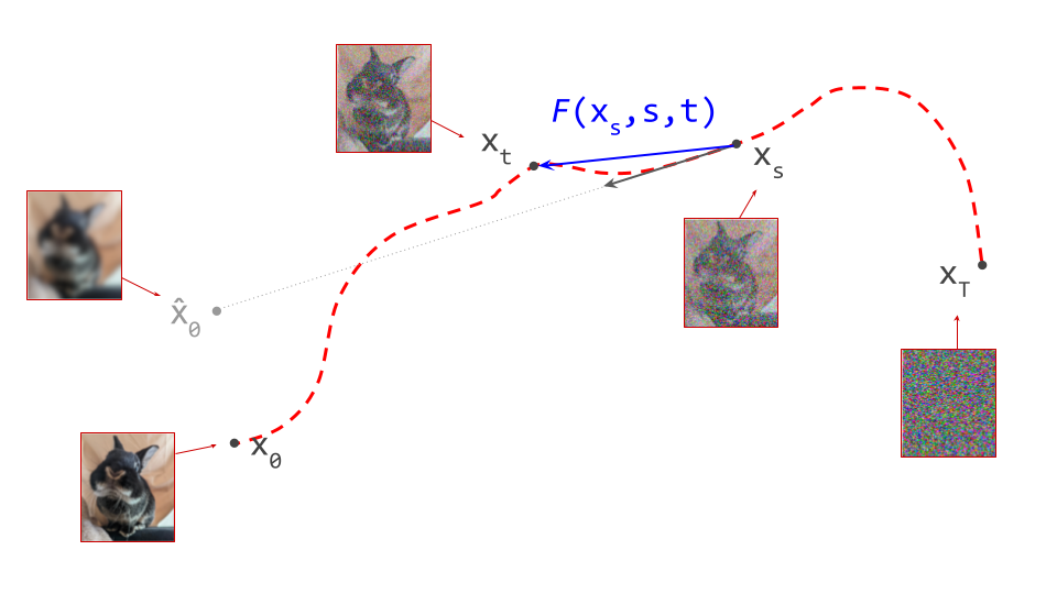
Cartography: mapping paths with a flow map

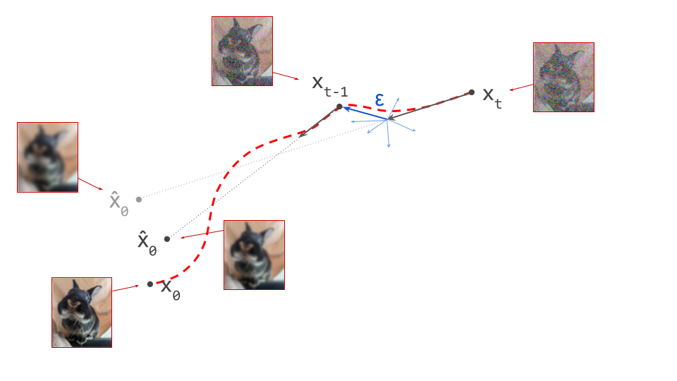
Learning to predict the tangent direction at any point on a path using a denoiser model is a way to fully characterise that path. But it is far from the only way to achieve that goal: flow maps offer a compelling alternative¹. At any point on a path, they can predict the location of any other point on that path.

Since we have already used \(f(\mathbf{x}_t, t)\) to describe a denoiser, let’s use \(F(\mathbf{x}_s, s, t)\) to describe a flow map. Note that it takes two time steps as input: \(s\) and \(t\) correspond to the source and target noise levels. Given a bijection between data and noise, the ideal flow map allows us to jump from anywhere on a path to anywhere else on that path: \(F(\mathbf{x}_s, s, t) = \mathbf{x}_t\). Usually we are interested in moving from noise towards data, so \(s > t\), but this doesn’t have to be the case. In practice, we will of course approximate this function with a neural network, just like we do with the denoiser when training a diffusion model.

In what follows, we will assume that we use the noise schedule commonly used in flow matching: \(\mathbf{x}_t = (1 - t)\mathbf{x}_0 + t\mathbf{\varepsilon}\) and \(T=1\), with \(\mathbf{\varepsilon} \sim \mathcal{N}(0, 1)\) (standard Gaussian noise). This is arguably the most popular choice nowadays, because it keeps things simple. While it is possible to derive everything in a more general setting (assuming only \(\mathbf{x}_t = \alpha(t) \mathbf{x}_0 + \sigma(t)\mathbf{\varepsilon}\) and arbitrary \(T\)), this complicates the maths, which makes it harder to follow. Note that we will stick to the original diffusion convention for the direction of time, so \(t=0\) corresponds to the data distribution, and \(t=1\) corresponds to noise (this is the opposite of the convention used in the flow matching paper). For more on the impact of these choices, check out my blog post on noise schedules.

With these choices, given a denoiser \(f(\mathbf{x}_t, t)\), which predicts the expected clean input \(\hat{\mathbf{x}}_0 = \mathbb{E}\left[\mathbf{x}_0 \mid \mathbf{x}_t\right]\), the tangent direction to the path or velocity \(\mathbf{v}_t\) is:

In the flow matching setting, we usually parameterise the neural network to predict the function \(v(\mathbf{x}_t, t)\) directly, instead of the expected clean input, but it is easy to get one from the other (because they are linear functions of each other and \(\mathbf{x}_t\)).

A flow map can now be constructed simply by integrating the velocity over a time interval:

This integral represents taking an infinite number of infinitesimally small steps along the path, accumulating the predicted tangent direction \(v(\mathbf{x}_t, t)\) as we go. If we add this integral to the starting point \(\mathbf{x}_s\), we end up in \(\mathbf{x}_t\).

In the typical case where we go from noise to data, \(s > t\), because \(t = 0\) corresponds to the data side in the diffusion convention, which makes the lower integration bound in this formula higher than the upper bound. This reflects how diffusion is defined in terms of a forward corruption process, and sampling from the data distribution actually means going backward. We defined \(\mathbf{v}_t\) to point from \(\hat{\mathbf{x}}_0\) towards \(\mathbf{x}_t\) by convention, so we want to follow this vector in the opposite direction to move towards the data side.

Some special cases are worth highlighting:

• If we set \(t=0\), we can directly jump from anywhere on the path to its end point at the data side: \(F(\mathbf{x}_s, s, 0) = \mathbf{x}_0\). Provided we can do this accurately, this enables sampling in a single step. This is precisely what consistency models¹¹ do. Flow maps are a generalisation of that idea, and we’ll discuss this connection in more detail later on.

• If we set \(s=t\), the interval over which we integrate has length zero, so the integral itself is zero, and therefore \(F(\mathbf{x}_t, t, t) = \mathbf{x}_t\).

• Although we are usually interested in traversing paths from noise to data, which implies \(t < s\), this does not have to be the case. We can use the same formulas to go in the other direction, by choosing \(t > s\). As an example, \(F(\mathbf{x}_s, s, 1)\) predicts the end point at the noise side of the path containing \(\mathbf{x}_s\).

Hopefully it is obvious that learning to predict the function \(F(\mathbf{x}_s, s, t)\) with a neural network is a harder task than learning to predict \(f(\mathbf{x}_t, t)\) – not least because it has two time step inputs instead of one. It provides a global characterisation of the paths between data and noise samples, rather than a strictly local one. This can also be much more practical: once we have a flow map, we don’t need to worry anymore about taking small enough steps during sampling to avoid falling off the path. In fact, if our neural network approximation is good enough, we can just sample noise \(\mathbf{\varepsilon}\) and take a single step, \(F(\mathbf{\varepsilon}, 1, 0)\) directly from \(s=1\) to \(t=0\) to arrive at \(\mathbf{x}_0\), and we’re done sampling! In the next section, we will discuss how to train flow map models.

Just like it is common to parameterise diffusion models to predict either the expected clean input \(\hat{\mathbf{x}}_0\) or the velocity \(\mathbf{v}_t\), there are two equivalent parameterisations for flow maps. The one we have described so far, \(F(\mathbf{x}_s, s, t)\), predicts the destination on the path, but we can also predict the average velocity or mean flow along the path¹²:

The relation between the two parameterisations is:

Here, the limiting case \(s = t\) yields \(V(\mathbf{x}_t, t, t) = v(\mathbf{x}_t, t)\): the average velocity over a length-zero interval is simply the instantaneous velocity. This shows that a flow map contains within it a denoiser, and therefore it can also be used as a standard diffusion model.

Given that it is possible to construct flow maps, one might be led to believe that they make diffusion models obsolete. The former are a strict generalisation of the latter, and the global view of paths between data and noise samples that they provide has many practical benefits. But as we will see, all the approaches that have been developed so far to construct this global view, work by bootstrapping from the local view provided by diffusion models. Sometimes this relationship is explicit, and sometimes it is less obvious, but it is always there. As ever in machine learning, there is no free lunch: while sampling using a flow map is cheaper than sampling from a diffusion model, training a flow map is significantly more involved, and often requires training a diffusion model first. Just like drawing an accurate map makes navigation a lot easier, but requires a lot more work up front!

Three notions of consistency

A flurry of different algorithms have been proposed to train flow maps. It turns out all these variants are ultimately based on one of three closely related consistency rules: compositionality, Lagrangian consistency and Eulerian consistency. In this section, we will cover each of these in turn, and then discuss how we can use them for flow map training.

Boffi, Albergo and Vanden-Eijnden originally developed the flow map framework and described these three rules (and training procedures derived from them) in two recent papers on flow map matching¹ and self-distillation². Although their work is rooted in the ‘stochastic interpolant’ perspective, I will not adopt this here and stick with a more traditional diffusion framing instead, as I believe more people are familiar with that.

Compositionality

The flow map \(F(\mathbf{x}_s, s, t)\) allows us to travel directly from \(\mathbf{x}_s\) on the path to \(\mathbf{x}_t\) on the same path. We can repeat the same procedure to travel farther along the path from there, using \(F(\mathbf{x}_t, t, u)\) to take us to \(\mathbf{x}_u\). But we could also have got there in one step, using \(F(\mathbf{x}_s, s, u)\). Either way of traversing the path should yield the same result:

In other words, flow maps are compositional. This is what I’m calling this property – it is a nonstandard term. I’m being stubborn about this, because I find the various names used in the literature to be ambiguous and confusing. You’ll see this called the ‘semigroup property’, the ‘shortcut property’, or ‘progressive matching / distillation’.

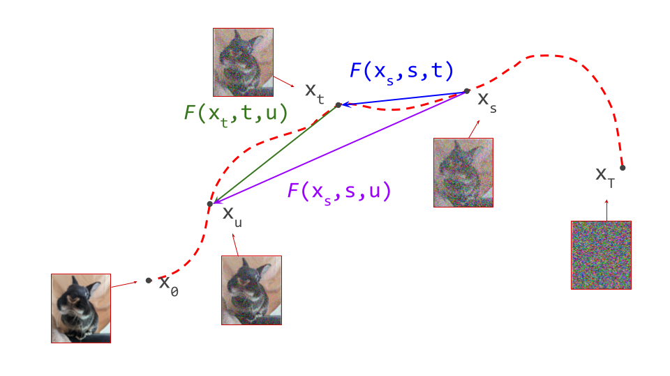
A corollary is that a flow map is its own inverse (with regards to its first argument):

In this case, we’ve assumed that the flow map is defined for both \(s > t\) and \(t > s\). Very often however, flow maps are only trained in one direction (\(s > t\), from high noise levels to low noise levels), because that is the relevant direction for sampling (moving towards the data distribution).

We can use compositionality to train a flow map by bootstrapping from a diffusion model. We start at \(\mathbf{x}_s\) and use the diffusion model to predict the next point on the path \(\mathbf{x}_t\), a short distance ahead. We can then use the fact that the flow map should always give the same answer, regardless of the starting point: \(F(\mathbf{x}_s, s, u) = F(\mathbf{x}_t, t, u)\), and as a special case, for \(t = u\): \(F(\mathbf{x}_s, s, t) = F(\mathbf{x}_t, t, t)\). By ensuring these equalities hold, we can transport information about the flow from smaller time intervals to larger time intervals.

The Lagrangian perspective: moving the goalposts

Another way to characterise the consistency of a flow map \(F(\mathbf{x}_s, s, t)\) is to study how its output changes as we gradually change \(t\), which indexes the destination (i.e. move the goalposts). This should result in the output \(\mathbf{x}_t\) travelling along the path. If we consider an infinitesimal change to \(t\), we can characterise what happens using the derivative:

In other words: the instantaneous change in the output of the flow map is the velocity. Intuitively this makes sense, as changing \(t\) means we are simply traversing the path, and the velocity is precisely the direction we should travel in to follow that trajectory.

We can expand the velocity \(\mathbf{v}_t = v(\mathbf{x}_t, t) = v(F(\mathbf{x}_s, s, t), t)\), and this gives us another way to bootstrap flow map learning from a diffusion model \(v(\mathbf{x}_t, t)\). We must simply ensure that the following equality holds everywhere:

where we have used that the total derivative of the flow map w.r.t. \(t\) is equal to the partial derivative, because the other arguments do not depend on \(t\): \(\frac{\mathrm{d}F}{\mathrm{d}t} = \frac{\partial F}{\partial t}\).

Another way of interpreting Lagrangian consistency is that it is just a special case of compositionality, where we have shrunk the second time interval to be infinitesimal: we let \(t \rightarrow u\) and look at the limiting behaviour. Let’s take the compositionality rule and replace \(u\) by \(t + \Delta t\) to make this more explicit:

This equation is also true when \(\Delta t = 0\):

Subtracting this special case from the original equation, and dividing by \(\Delta t\), we get:

Finally, we take the limit as \(\Delta t \rightarrow 0\), and use the definition of the derivative:

To simplify the left hand side, we recall the original flow map definition, \(F(\mathbf{x}_s, s, t) = \mathbf{x}_s + \int_s^t v(\mathbf{x}_\tau, \tau) \mathrm{d} \tau\), and take the corresponding derivative:

where we have used that \(\frac{\mathrm{d}}{\mathrm{d}t} \mathbf{x}_s = 0\), and the fundamental theorem of calculus. Applying this simplification, we once again find:

The Eulerian perspective: eyes on the prize

Instead of looking at the impact of changing the target time step \(t\), we can also study what happens when \(s\) changes, i.e. the starting point. At first glance, this looks even simpler:

When we change the starting point, but the target time step \(t\) remains the same, the destination should not change at all. Therefore, its derivative must be zero. Easy enough, right? This apparent simplicity is deceptive, however. We now have two inputs that depend on \(s\): the source time step \(s\), and also our actual starting position in the input space, \(\mathbf{x}_s\).

Because two of our three function inputs now depend on \(s\), we need to use the multivariate chain rule to work this out:

This is basically a combination of two changes: the change in the input space resulting from the change to the starting time step \(s\), and the change to the starting time step itself.

We note that \(\frac{\mathrm{d} \mathbf{x}_s}{\mathrm{d}s} = v(\mathbf{x}_s, s) = \mathbf{v}_s\), and obtain yet another equality that enables us to bootstrap flow map learning from a diffusion model, by ensuring it holds everywhere:

As with Lagrangian consistency, we can interpret Eulerian consistency as a special case of compositionality. This time, we shrink the first time interval to be infinitesimal instead, letting \(s \rightarrow t\). Let’s recap the compositionality rule one more time, and substitute \(t\) with \(s + \Delta s\):

Because \(\Delta s\) is very small, we can use the following approximation:

where we have assumed that \(v(\mathbf{x}_\tau, \tau)\) remains constant over the integration interval. Since we plan to let \(\Delta s \rightarrow 0\), this is a valid assumption. We now have:

We now perform a first-order multivariate Taylor expansion around \((\mathbf{x}_s, s)\) on the left hand side, to get:

Note that \(F(\mathbf{x}_s, s, u)\) appears as the first term, and also on the right hand side of our previous equation, so these cancel out. We are left with:

Now just divide out \(\Delta s\) to recover the Eulerian consistency rule:

Although we didn’t explicitly take a limit \(\Delta s \rightarrow 0\) anywhere, we did rely on approximations that are only valid when it is very small.

Eulerian and Lagrangian consistency are ultimately just different perspectives of the same thing, using different reference frames. For Lagrangian consistency, we focus on a specific noisy input example, and track how the flow map’s output evolves over time. For Eulerian consistency, we fix the target time step and assess how things change as the input changes. If the flow is a river, it’s basically the difference between sitting in a canoe, following its path (Lagrangian), and standing on a bridge, looking down (Eulerian).

Constructing loss functions from equalities

The equations describing these three consistency rules can feel somewhat tautological, almost trivial even: it is clear that they must be true for any valid flow map. But neural networks are flexible enough to learn almost any function of three inputs, \(\mathbf{x}_s\), \(s\) and \(t\), and most of these possibilities will not be consistent in the way that a valid flow map should be. When learning a flow map, it is therefore useful to explicitly enforce the consistency rules.

It turns out that any of them will do: if a function adheres to any of the three consistency rules we have just discussed, in combination with the right boundary conditions, it is automatically a valid flow map. This actually gives us a lot of options for constructing loss functions to train flow maps with.

The consistency rules are all equalities. Turning these into loss functions is pretty straightforward: move all terms over to the left hand side, so that the right hand side is zero. The left hand side is now a residual, which measures how far away we are from achieving consistency. Then, simply penalise the residual, so that it ends up as close to zero as possible when the loss is minimised. The most straightforward way to achieve that is to simply square the left hand side, and average over all possible time step combinations (and the training dataset) to obtain a loss function.

For the three consistency rules, we get, respectively:

The minima of all three of these loss functions guarantee consistency. Even if we cannot perfectly minimise these functions in practice, we can usually get close enough for things to work as expected.

To learn something useful, we constrain \(F(\mathbf{x}_t, t, t) = \mathbf{x}_t\), and ensure that \(v(\mathbf{x}_t, t)\) corresponds to a meaningful velocity. This can be achieved by first training a diffusion model and using that as a reference (i.e. distillation), but there are also other ways to constrain the implied velocity, which enable training flow maps from scratch (see section 4).

Note that squaring the residual is an arbitrary choice, to some extent. We could also penalise its absolute value, or use something more exotic like the Huber loss. In some cases, as we will see later, we can even use the categorical cross-entropy. The mean squared error (MSE) approach has some practical advantages though: it is relatively easy to optimise by gradient descent, and essential for some from-scratch training methods to work (see section 4.2).

To backprop or not to backprop?

Taking a closer look at these loss functions, there are are some things that are bit unusual about them:

• two of them contain derivatives of the function \(F\) that we are trying to learn (Lagrangian and Eulerian). This implies that gradient-based learning could potentially involve higher-order derivatives.
• the other variant involves multiple sequential applications of \(F\), potentially requiring sequential forward and backward passes during training.

Unlike most loss functions used in machine learning, which measure the difference between a model prediction and a static target (the ‘ground truth’), these ones involve moving targets and are self-referential. In theory, gradient-based optimisation doesn’t care about this: it just tries to find an optimum of whatever function you throw at it (usually a local optimum). But by casting flow map training into this more traditional machine learning framework with static targets, we can actually overcome some hurdles, like avoiding having to calculate higher-order derivatives.

Stemming the flow (of gradients)

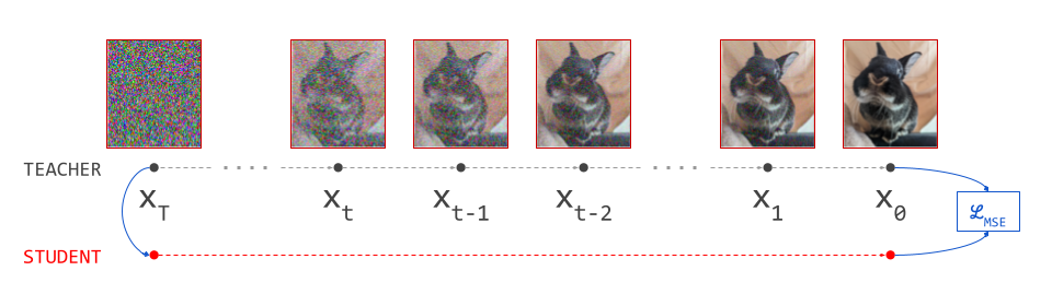
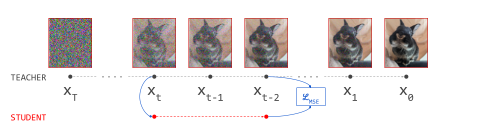
We can take inspiration from representation learning, where these types of self-referential loss functions with moving targets have become increasingly common^{13 14}. Here, one network learns to mimic the output of another, like the student and teacher in distillation. The teacher is constructed using the same parameters as the student. Often, an exponential moving average (EMA) of the parameters is used, and no gradients are backpropagated through the teacher side of the loss, which helps avoid collapse to a degenerate solution.

The same kind of tricks can be used to stabilise and simplify flow map training. We can wrap portions of the loss in a stop-gradient operation. This blocks gradient flow during backpropagation, and acts as a pass-through otherwise:

where \(\mathrm{sg}[\cdot]\) indicates the stop-gradient operation. Anything that is wrapped inside will be treated as constant for the purpose of backpropagation, so we avoid having to backpropagate through \(\nabla_{\mathbf{x}_s} F(\mathbf{x}_s, s, t)\), for example. Similarly in the compositional case, we can use a stop-gradient operation to avoid sequential backward passes:

This has an elegant interpretation: we calculate a target using two sequential flow map steps, treat it as ground truth and freeze it, and then update the flow map to learn how to get there in one step.

Since any part of the loss wrapped inside a stop-gradient operation is effectively treated as static (even if it technically isn’t), we can sometimes stabilise training by using EMA parameters to calculate it. This ensures that it varies more slowly over the course of training, which makes the implicit assumption that it is static less egregious.

Introducing the stop-gradient operation has an interesting implication: the ‘gradient’ direction calculated by backpropagating only through part of the loss, is not actually a gradient direction! At least, it is not the gradient direction of the loss that we are trying to optimise – it could still be a valid gradient for another loss function, for all we know. It is sometimes referred to as a semigradient². This means that some theoretical guarantees about gradient-based optimisation go out of the window. Luckily, when done with care, abandoning the safety of theoretical grounding does not seem to cause any major problems in practice (as is so often the case with neural networks), but it is worth being aware of.

The loss variants given above are just examples: exactly which parts of the loss expressions are wrapped in stop-gradient operations, or are stabilised by using EMA parameters, is what distinguishes various flavours of flow map training. We will explore this design space extensively in section 5.

The ‘average velocity’ perspective

At this point, it is useful to recall the average velocity parameterisation of flow maps, which we previously discussed in section 1.3. This is because it interacts in interesting ways with the derivatives in the Lagrangian and Eulerian consistency rules:

We can express the Lagrangian consistency rule in terms of \(V\) by substitution:

We have not performed the substitution for the first argument of \(v\), as this would not allow us to simplify anything anyway. Now we can work out the time derivative on the left hand side, which requires the product rule:

Note how in addition to its time derivative, \(V\) itself appears in this expression. Rearranging the terms to isolate \(V\), we get:

We can interpret this as follows: the average velocity over the time interval between \(s\) and \(t\) is the velocity at the endpoint, minus a correction term involving the derivative of the average velocity itself w.r.t. the target time step \(t\). When we use this expression to construct a loss, we can wrap the entire right hand side in a stop-gradient operation. That means we don’t have to worry about backpropagating through the time derivative, and no higher-order differentiation is needed to optimise the loss.

We can do the exact same thing with the Eulerian consistency rule:

Using the product rule (twice), we get:

Rearranging to isolate \(V\), we get:

This expresses the average velocity as the velocity at the starting point, plus a correction term involving the derivative of the average velocity itself w.r.t. the source time step \(s\). We can once again wrap the entire right hand side in a stop-gradient operation, which forms the basis of MeanFlow¹²:

Forward- and reverse-mode differentiation

Modern frameworks for neural network training calculate gradients for you, so you rarely need to worry about them, but the automatic differentiation machinery that makes this possible is quite intricate.

To calculate gradients for a deep computation graph, there are two main methods: forward-mode and reverse-mode differentiation. They traverse the graph from input to output, and from output to input respectively. The choice between them comes down to the dimensionality of the input and output: if the output is higher-dimensional than the input, forward mode is more efficient. In the other case, reverse mode wins out. When training a neural network, the input is usually high-dimensional, but the ultimate output of the computation graph we are differentiating is almost invariably a single loss value. That is a scalar, so the output dimensionality is much lower than the input dimensionality, and reverse mode is the right choice. This is what these frameworks will use by default.

Forward mode does make an occasional appearance, though; it can be used to efficiently compute Jacobian-vector products (JVPs). Such a product occurs in the Eulerian consistency rule:

The Jacobian of \(V\), which consists of all its partial derivatives, is multiplied by the so-called tangent vector \([v, 1, 0]\). In JAX, we can use jax.jvp to calculate this. It efficiently computes both the forward pass and the derivative at the same time, and avoids explicitly materialising the full Jacobian matrix in memory. That’s not a luxury, because it is massive: \(V\) has the same shape as \(\mathbf{x}_s\), so if they are both vectors of size \(K\), then \(\frac{\partial V}{\partial \mathbf{x}_s}\) is a \(K \times K\) matrix!

Finite-difference approximations

Instead of stopping gradient flow altogether, another common trick to avoid dealing with derivatives is to replace them with finite-difference approximations. We can use the definition of the derivative:

Here, \(\Delta x\) is the finite difference. As long as it is small, the approximation can be quite good. Small values are prone to causing issues with floating point precision (especially nowadays, with low-precision neural network training being highly in vogue), so care needs to be taken when using this approach.

Remember how we derived the Lagrangian and Eulerian consistency rules from the compositionality rule by shrinking one of the time intervals to be infinitesimal? Applying a finite difference approximation to either of them would effectively make that interval finite again. This can make classification of methods according to the consistency rule they are based on somewhat ambiguous.

Practical considerations

It is worth asking if we really need all this mucking about with gradients. Why is it a problem to just backpropagate through everything? Modern frameworks certainly make it possible and even easy in the vast majority of cases, but that doesn’t mean it is always a good idea:

• Calculating higher-order derivatives can be costly, in terms of the number of floating point operations (FLOPS), but also and especially in terms of memory. It often involves keeping around large tensors for a long time, because they get reused in multiple places in the computation graph.

• Usually, higher-order derivatives of modern neural networks are not very meaningful. The second order derivative captures curvature, which often doesn’t vary smoothly across the input space. As an extreme example, a network with only ReLU nonlinearities is effectively piecewise linear, so its curvature is zero almost everywhere. This is also why we don’t typically parameterise diffusion models as the gradient of a scalar energy function, even though we definitely could¹⁵.

• More and more often, we use specialised fast kernels for certain operations (e.g. FlashAttention¹⁶). These tend to come with an equally efficient implementation of the backward pass, to support training. Forward-mode differentiation and higher-order derivatives usually aren’t implemented, requiring fallback to slower implementations.

Different implementations of flow map training will require different numbers of forward and backward passes for each training iteration (e.g. a finite difference approximation usually replaces a backward pass with two forward passes), and may or may not require forward-mode differentiation or higher-order derivatives. A notable case is Terminal Velocity Matching¹⁷ (TVM), an implementation based on Lagrangian consistency which does not make use of stop-gradient operations or any other approximations to avoid higher-order derivatives. The authors explicitly mention developing a custom attention kernel to support this. We will discuss various implementations in more detail in section 5.

Training flow maps from scratch

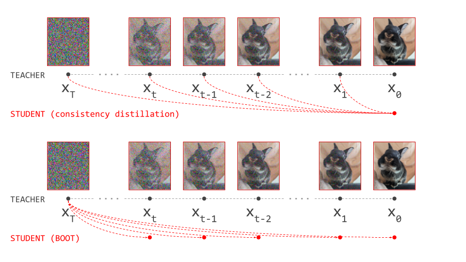
Building a flow map to describe paths between noise and data samples requires some form of bootstrapping: for example, training a diffusion model provides us with the velocity \(v(\mathbf{x}_t, t)\), which is by itself sufficient to completely describe said paths. We can then use that as a starting point for flow map training, which effectively turns it into a form of distillation.

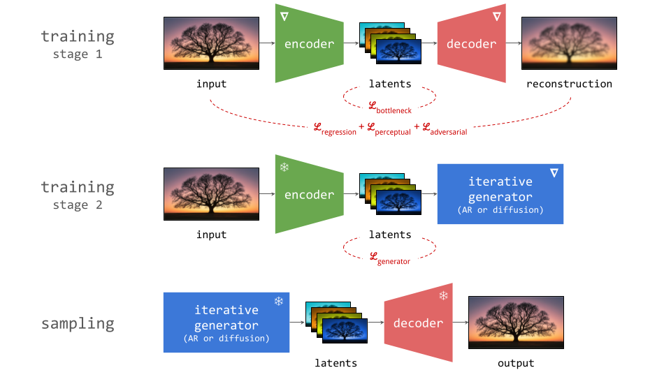
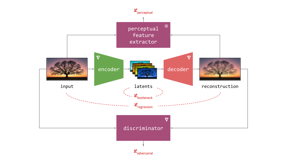
But what if we want to train a flow map from scratch? There are many good reasons to prefer a single-stage training process. Any sequential dependency adds a great deal of complexity, which we should only tolerate if it significantly improves the quality of the end result (incidentally, this is why we tolerate it in the case of latent diffusion).

Self-distillation

As previously mentioned, a flow map parameterised by the average velocity contains within it a velocity predictor as a special case: \(V(\mathbf{x}_t, t, t) = v(\mathbf{x}_t, t)\). So if we ensure that we occasionally sample \(s = t\) during training, and combine the consistency-based loss function of our choice with the standard diffusion loss applied to those cases, we don’t need a pre-trained model that provides ‘ground truth’ for \(v(\mathbf{x}_t, t)\). By balancing both losses, the model will simultaneously learn both the instantaneous velocity as well as its integral over finite time step intervals. As an example, we can combine the Lagrangian consistency loss with the diffusion loss:

Note that we have also substituted the appearance of \(v(\mathbf{x}_t, t)\) in the Lagrangian consistency loss term with \(V(\mathbf{x}_t, t, t)\) to enable from-scratch training.

We could also use this dual loss setup in combination with a pre-trained diffusion model, substituting \(\mathbf{\varepsilon} - \mathbf{x}_0\) with its velocity estimate to reduce the variance of the diffusion loss term, but this is not strictly necessary. Even if we don’t, it makes sense to interpret this as a form of self-distillation²: the model is simultaneously being trained as a teacher and being distilled into itself.

My own experience with neural network training setups where teacher training and student distillation are simultaneous rather than sequential, is that they can work pretty well in practice (my colleagues and I used this idea for representation learning at some point¹⁸). Results are usually as good or almost as good as having two sequential training stages (first the teacher, then the student), but without a lot of the hassle caused by the sequential dependency.

Marginal-from-conditional learning

Some flow map training formulations admit an alternative approach, which requires only a single consistency-based loss to train from scratch. To understand how this is possible, it is worth revisiting how diffusion training works: a denoiser learns to predict \(\mathbb{E}\left[\mathbf{x}_0 \mid \mathbf{x}_t\right]\), even though we supervise it with samples from \(p(\mathbf{x}_0, \mathbf{x}_t)\) during training. It is never directly supervised to predict the conditional expectation, but because it is forced to make a single prediction across all possible samples of \(p(\mathbf{x}_0, \mathbf{x}_t)\), it automatically lands on the expectation as the best way to minimise the overall error. This is sometimes known as the marginalisation trick, because it enables learning the marginal velocity from velocities conditioned on \(\mathbf{x}_0\)¹⁹.

How can we apply this same trick to flow map training? There are two different approaches to make this work, both starting from the Eulerian consistency rule: MeanFlow¹² and improved MeanFlow ²⁰ (iMF). Let’s look at the original MeanFlow approach first. Using the average velocity formulation, we have:

If we treat the right hand side of this equality as the target for learning, and wrap it in a stop-gradient operation, we can substitute the marginal velocity \(v(\mathbf{x}_s, s)\) by the conditional velocity, which is simply \(\mathbf{\varepsilon} - \mathbf{x}_0\) (as in diffusion). This will leave the minimum of the MSE loss unchanged. It’s worth taking a moment to dissect exactly why we are allowed to do this. It hinges on four important features:

• We use the mean squared error as the loss.
• The velocity is evaluated at the current noisy input \(\mathbf{x}_s\).
• The prediction target is linear in the velocity \(v(\mathbf{x}_s, s)\).
• The stop-gradient operation ensures that the resulting update direction remains linear in the velocity.

Let’s call the residual \(R\): this is the difference between the left hand side and the right hand side of the consistency rule. \(R\) is linear in \(v(\mathbf{x}_s, s)\). The loss function we are minimising is then simply \(\mathbb{E}\left[R^2\right]\). If we take the gradient of this loss function with respect to our model parameters \(\theta\), we get:

But because the prediction target is wrapped in a stop-gradient operation, this is not actually the update direction we use. Instead, we end up with:

because \(V(\mathbf{x}_s, s, t)\) is the only part of \(R\) that sits outside the stop-gradient operation. Therefore, the update direction \(\widetilde{G}_\theta\) is also linear in the velocity. If we swap out \(v(\mathbf{x}_s, s)\) for \(\mathbf{\varepsilon} - \mathbf{x}_0\), the expectation operator ensures that we still get exactly the same result, because the expectation is conditional given \(\mathbf{x}_s\).

Note that this would not be the case if it weren’t for the stop-gradient operation: the ‘proper’ gradient \(G_\theta\) contains the product of \(R\) and \(\nabla_\theta R\), both of which depend on the velocity, so this update direction is not at all linear in the velocity, and the marginal-from-conditional learning trick would completely break down!

If the velocity were evaluated anywhere else than \(\mathbf{x}_s\), it also wouldn’t work: substituting the marginal velocity with the conditional velocity \(\mathbf{\varepsilon} - \mathbf{x}_0\) only works because we are calculating a conditional expectation given \(\mathbf{x}_s\). This is why we cannot give the Lagrangian consistency rule the same treatment: it requires evaluating the velocity at \(\mathbf{x}_t = F(\mathbf{x}_s, s, t)\). So even though the prediction target is also linear in the velocity, and we can use the stop-gradient operation to ensure that the update direction remains linear in the velocity, the expectation is conditioned on the wrong variable for the substitution to work.

It is fair to say that the stop-gradient operation in MeanFlow is doing double duty: it avoids higher-order differentiation (no backprop through derivatives), and it enables marginal-from-conditional learning. At a glance, it looks like a tweak to make training more efficient, but it is actually crucial for training to work at all.

For improved MeanFlow (iMF), we start from the same average velocity formulation of the Eulerian consistency rule, but with a twist: we make \(V(\mathbf{x}_s, s, t)\) and \(v(\mathbf{x}_s, s)\) swap sides:

Now we have an expression for the instantaneous velocity \(v\) at the starting point \(s\) in terms of the average velocity \(V\) over the interval between \(s\) and \(t\). It is unfortunately self-referential, as the instantaneous velocity appears inside the Jacobian-vector product (JVP) on the right hand side. But recall that the instantaneous velocity is also just the average velocity over an empty interval: \(v(\mathbf{x}_s, s) = V(\mathbf{x}_s, s, s)\), so:

Now, we can interpret the expression the right side as simply a reparameterisation of a standard diffusion or flow matching model, and train it as if it is one. In other words, we define:

(Confusingly the iMF paper uses the notation \(V\) for this, but I have already used that letter for the average velocity. Sorry!) Note the stop-gradient operation wrapping the calculation of the JVP. We can use \(W\) as the predictor in the usual MSE loss:

Training the ‘diffusion model’ \(W\) now forces \(V\) to learn the average velocity across intervals, and therefore, a full flow map, purely through its parameterisation. How neat is that?

Technically, we don’t even need any stop-gradient trickery to make this work, although in practice, the JVP is still wrapped in a stop-gradient operation to avoid higher-order differentiation. Unlike in traditional MeanFlow, however, the stop-gradient is not at all necessary for the method to work correctly! Aside from being more elegant, the improved MeanFlow loss also tends to have much lower variance in practice.

Flow maps in practice

Now that we have established what flow maps are, how they relate to diffusion models and how to train them, let’s take a closer look at some concrete implementations described in the literature. As usual, this is an opinionated selection of papers, and I do not purport to give an exhaustive overview. Feel free to drop any glaring omissions (or just interesting related work) in the comments below. This is going to be relatively dry, so I won’t be offended if you skip ahead to the end of the section, where I will summarise everything in a table.

If you are planning to read any of the papers mentioned, it is worth being aware of some of the notational variations you might encounter:

• The direction of time can be from data (\(t=0\)) to noise (\(t=1\)), following the diffusion convention, or from noise (\(t=0\)) to data (\(t=1\)), following the flow matching convention. I have stuck with the former, but many papers use the latter instead.
• The source and target time steps are sometimes given in reverse order, specifying the target first, and then the source, i.e. \(F(\mathbf{x}_s, t, s)\) instead of \(F(\mathbf{x}_s, s, t)\). Sometimes the target time step is fixed, and therefore omitted (as in consistency models¹¹): \(F(\mathbf{x}_t, t)\).
• The time steps can be arguments to a function (e.g. \(F(\mathbf{x}_s, s, t)\)), but they are often specified as indices instead (e.g. \(F_{s,t}(\mathbf{x}_s)\)). I prefer explicit function arguments, because we often need to take (partial) derivatives with respect to these time steps.
• Functions representing flow maps and diffusion models can use lower case letters, upper case letters or Greek letters. Time steps are often \(s\) and \(t\), \(t\) and \(s\) or \(t\) and \(r\), there is no standard convention. I like \(s\) for ‘source’ and \(t\) for ‘target’, so that’s what I’ve stuck with, but many papers actually use them the other way around!

There were several instances during the writing of this blog post where these discrepancies got me hopelessly confused. If you look out for them and spend some time to make sure you are interpreting the notation correctly, you might save yourself a lot of hassle. It is also important to keep in mind the choice of parameterisation (flow map \(F\), average velocity \(V\), or something else). As we have seen before when discussing the consistency rules, this choice can make the formulas look quite different.

Training a diffusion model is remarkably simple, when you think about it: you only need very basic concepts such as Gaussian noise and the the mean squared error loss. As we have already seen, training flow maps is quite a bit more involved by comparison. Often, it is also more costly, requiring multiple passes through the model to perform a single training step.

Lagrangian methods 🐱

Boffi et al. describe Lagrangian map distillation¹ (LMD). Given a pre-trained teacher model that predicts the velocity, minimise:

They suggest using forward-mode differentiation (JVP with tangent vector \([0, 0, 1]\)) to efficiently calculate \(\frac{\partial}{\partial t} F(\mathbf{x}_s, s, t)\) and \(F(\mathbf{x}_s, s, t)\) simultaneously. Note the lack of stop-gradient operations, so minimising the loss function requires higher-order differentiation. Although the loss is expressed in terms of \(F\), they suggest predicting \(V\). For from-scratch training, a self-distillation variant can be constructed² by replacing the velocity with the flow map’s own prediction (note the introduction of a stop-gradient operation), and combining it with a standard diffusion loss (see section 4.1):

Align Your Flow²¹ proposes a similar distillation approach (AYF-LMD), but arrives at it from a compositional perspective: taking a large step from \(s\) to \(t\) should be equivalent to taking slightly smaller step from \(s\) to \(t - \Delta t\), and then using the teacher model to go the rest of the way to \(t\) (i.e. a diffusion sampling step):

They construct a loss from this identity, by wrapping the right-hand side in a stop-gradient operator and squaring the residual, and then taking the limit for \(\Delta t \rightarrow 0\). They show that this recovers \(\mathcal{L}_\mathrm{LMD}\) (except of course for the stop-gradient, which helps avoid higher-order differentiation). Although they note it is more stable than their Eulerian approach (see section 5.2) in toy experiments, they also point out that it fails to produce good results on real images.

Terminal Velocity Matching¹⁷ (TVM) follows a similar recipe, but targets training from scratch using self-distillation (see section 4.1). Their ‘terminal velocity condition’ is precisely the Lagrangian consistency rule, and the TVM loss consists of a Lagrangian consistency term and a flow matching (diffusion) term. Interestingly, they suggest using a stop-gradient operation on the weights for some of the model invocations, and even exponentially averaged (EMA) weights for one of them. However, they do not apply this operation to the derivative term that appears in the consistency loss term, so higher-order differentiation is required for training. They point out that this necessitates a custom FlashAttention kernel, which they have open-sourced, as well as several architecture and optimisation tweaks, such as a Lipschitz continuity constraint.

FreeFlow²² figures out a clever way to make flow map distillation entirely data-free, using Lagrangian consistency as a starting point. They exclusively draw samples from the noise distribution to successfully distill a diffusion model into a flow map. They also make a compelling argument for why you would want to eliminate the requirement of a training data distribution altogether: it might not actually be representative of the samples the diffusion model is able to generate, even if it was trained on that distribution itself! This can be because of interventions like classifier-free guidance, but also simply because the model has learnt to generalise beyond the data distribution. And sometimes, the original data distribution simply isn’t accessible at the time of distillation.

It is clearly suboptimal if the data distribution used to perform flow map distillation isn’t representative of the sampling trajectories we are trying to model. But how can you train a neural network without data? They achieve this feat by combining two ingredients:

• A Lagrangian consistency distillation loss, using the average velocity formulation, with the source time step anchored to \(s = 1\). They always start from pure noise \(\mathbf{\varepsilon} \sim \mathcal{N}(0, 1)\) and minimise (using a finite-difference approximation for the derivative):

• An auxiliary denoiser model is concurrently trained on one-step flow map samples, \(F(\mathbf{\varepsilon}, 1, 0)\), by renoising them according to the original corruption process. They then compare the velocity predicted by this denoiser to the teacher velocity, and use the discrepancy between the two to update the flow map. This helps to ground the distribution \(p(\mathbf{x}_0)\) implied by the flow map.

They show that each component in isolation is not sufficient to learn a good flow map model: using only the auxiliary denoiser is prone to collapse, and using only the Lagrangian consistency loss is prone to error accumulation. FreeFlow is closely related to BOOT²³, an earlier data-free distillation method based on Lagrangian consistency, which I have previously discussed on this blog.

Physics Informed Distillation²⁴ (PID) draws inspiration from physics-informed neural networks (PINNs), where people have been using neural networks to learn the solution operator of differential equations for a long time. Those methods are just as applicable to the ODE used for deterministic sampling from diffusion models, as they are to ODEs that describe physical phenomena. This yields another data-free distillation variant based on Lagrangian consistency. Like in FreeFlow, the derivative is handled by using a finite-difference approximation, but here, the stop-gradient operation only wraps the teacher velocity:

They mention that avoiding backpropagation through the teacher is essential, because it enables the student to exploit weaknesses in the teacher (a similar phenomenon to adversarial examples).

Eulerian methods 🐔

Eulerian map distillation¹ (EMD) uses a loss that is straightforwardly derived from Eulerian consistency (using velocity estimates from a pre-trained teacher model):

As with LMD, a self-distillation version can be constructed² by replacing the velocity with the flow map’s own prediction, and combining it with a standard diffusion loss. A stop-gradient operation is added to wrap the spatial part of the Jacobian \(\nabla_{\mathbf{x}_s} F(\mathbf{x}_s, s, t)\).

Align Your Flow²¹ also features an Eulerian distillation method (AYF-EMD). As with the Lagrangian version, they start by comparing a large step and a slightly smaller one:

where \(\mathbf{x}_{s + \Delta s} = \mathbf{x}_s + \Delta s \cdot v(\mathbf{x}_s, s)\). The right-hand side is wrapped in a stop-gradient operation, and the squared residual is used as the loss. They show that letting \(\Delta s \rightarrow 0\) recovers \(\mathcal{L}_\mathrm{EMD}\), once again excepting the stop-gradient operation, which in this case helps avoid backpropagation through the spatial part of the Jacobian. For their best results, they combine this with autoguidance²⁵ applied to the teacher, a warmup training phase with linearity regularisation, and an adversarial finetuning phase where the EMD loss is combined with an adversarial loss.

Solution Flow Models²⁶ (SoFlow) follow a very similar recipe, with two key differences:

• They focus on learning flow maps from scratch, and use self-distillation as the mechanism to do so (whereas AYF is focused on distillation from a pre-trained diffusion model);
• The Jacobian-vector product is avoided through a finite-difference approximation (\(\Delta s\) is small but finite, rather than infinitesimal), with one side of it wrapped in a stop-gradient operation.

To make the finite difference approximation work well in practice, they tweak the loss weighting and use a curriculum to gradually decrease \(\Delta s\) over the course of training.

Flow-anchored consistency models²⁷ (FACM) are also similar to AYF in spirit, but use an interesting trick to improve training stability, which they call ‘flow anchoring’. The base version of FACM considers \(t=0\) only: the target time step is fixed, as in consistency models. They then extend the range of the source time step \(s\) from \([0, 1]\) to \([0, 2]\). When \(s > 1\), the model is expected to operate as a denoiser. This results in a single model with a flow map mode and a denoiser mode, which shares parameters across these two tasks. This is said to ‘anchor’ the parameters of the model: the auxiliary denoiser task acts as a regulariser for flow map learning.

The flow anchoring parameterisation is combined with an efficient JVP implementation. They also consider a version where \(t\) is allowed to vary, enabling full flow map learning. Interestingly, in that setting, the model learns a denoiser twice: once for the auxiliary denoiser task (\(s > 1\)), and once for the flow map task when \(t = s\). Despite the apparent redundancy, the auxiliary task still seems to be helpful even in this case.

Unlike the preceding approaches, MeanFlow¹² (MF) does not rely on (self-)distillation, but on marginal-from-conditional learning, just like standard diffusion or flow matching models. The mechanics of this were already explained in a previous section (including the improved MeanFlow²⁰ variant). The practical implementation of MF involves adaptive weighting to avoid volatility as \(s\) and \(t\) get close to each other. In addition, the \(s = t\) case is significantly oversampled during training to keep the model grounded.

Many variants and extensions of MeanFlow have been explored. Here are a few:

• AlphaFlow²⁸ suggests a curriculum learning approach, smoothly interpolating from learning the instantaneous velocity (flow matching) to the average velocity (MF) over the course of training.

• Decoupled MeanFlow²⁹ (DMF) proposes an architectural tweak: condition the earlier layers of the network only on the source time step \(s\), and the later layers only on the target time step \(t\). This makes it quite straightforward to adapt a pre-trained denoiser into a MeanFlow model: simply decouple the time embeddings for the earlier and later layers, and then fine-tune. They also suggest using a Cauchy variant of the MF loss to supress outliers.

• Rectified MeanFlow³⁰ starts from the following observation: if all paths between data and noise are completely straight, the instantaneous velocity and average velocity (over any interval) coincide everywhere! The less curved the paths, the easier it will be to adapt a denoiser into a MeanFlow model. They suggest combining a single reflow¹⁰ stage with MF training.

• Pixel MeanFlow³¹ (pMF) notes that the computational benefits of generative modelling in latent space start to wane when your model needs very few steps to produce good samples. At that point, the relative simplicity of operating directly in input space might be preferable, so they explore how to adapt iMF for this setting.

Compositional methods 🐶

Shortcut models³² use a loss function in terms of the average velocity \(V\) based on the compositional consistency rule, grounded with self-distillation:

where \(\hat{V}_\mathrm{s + 2h} = \frac{V(\mathbf{x}_s, s, s + h) + V(\hat{\mathbf{x}}_{s + h}, s + h, s + 2h)}{2}\) and \(\hat{\mathbf{x}}_{s + h} = \mathbf{x}_s + h V(\mathbf{x}_s, s, s + h)\). This looks a bit gnarly at first, but it is simply saying that the average velocity over a time interval of length \(2h\) should be the mean of the average velocities over two intermediate time intervals with length \(h\). This strategy of bootstrapping by doubling the step size is very similar to progressive distillation³³. Note that no derivatives feature anywhere in the loss.

SplitMeanFlow³⁴, which might sound like it belongs in the previous section, is actually a generalisation of shortcut models, where the time intervals that are composed are not restricted to be the same length. They focus on distillation instead of from-scratch training. Boffi et al. recover the self-distillation variant as Progressive self-distillation² (PSD).

Flow Map Matching¹ (FMM) takes a slightly different approach: recall that compositionality implies that a flow map is its own inverse, \(F(F(\mathbf{x}_s, s, t), t, s) = \mathbf{x}_s\). Taking the partial derivative w.r.t. \(s\), we also get:

Combined, these two equalities are used to construct the FMM loss:

Note the use of marginal-from-conditional learning for the first term, which enables from-scratch flow map training. Unfortunately, this term also reintroduces a time derivative, but since it is a partial derivative w.r.t. \(s\), it does not require backpropagation into \(F(\mathbf{x}_s, s, t)\). They find that this method works best when the time interval \(\mid t - s \mid\) is restricted so it is not too large, which means it is not suitable for learning to sample in one step.

To address the latter, they also suggest Progressive Flow Map Matching (PFMM):

where \(F_\mathrm{pre}\) represents a pre-trained flow map across a limited time interval. This is arguably the purest application of the compositional consistency rule, but it does require a pre-existing partial flow map to work (which can be obtained through FMM or another method).

What about consistency models?

There is a long line of work around consistency models dating back to 2023. I wrote about some of it in a previous blog post. The original Consistency Models paper¹¹ (CM) set off something of a chain reaction, as people came to realise that predicting velocities is only one of many ways to characterise paths between noise and data. Although the ‘flow map’ framing did not come until much later, I have chosen to use it for this blog post, because I think it provides a helpful framework for understanding how all of this work relates to each other. Many recent works have also adopted it.

That said, it is worth taking a moment to see how some of these original works fit into the modern framework. Consistency Distillation (CD) produces a flow map with the target time step anchored to \(t=0\) (data side):

with \(\hat{\mathbf{x}}_{s - \Delta s} = \mathbf{x}_s - \Delta s \cdot v(\mathbf{x}_s, s)\), the output of a single Euler sampling step over the time interval \(\Delta s\). In this way, the loss quite literally propagates predictions from small time steps (closer to data) to large time steps (closer to noise). Taking the limit as \(\Delta s \rightarrow 0\) recovers Eulerian map distillation. Consistency Training (CT) enables from-scratch learning by replacing the velocity \(v(\mathbf{x}_s, s)\) with the conditional velocity, but unlike MeanFlow, this now results in a biased estimate. They show the bias goes away as \(\Delta s \rightarrow 0\).

CD and CT construct a partial flow map (for \(t=0\) only), so sampling from consistency models in multiple steps involves reinjecting noise, because every step fully denoises the input. Several follow-up works improved upon the original training recipe, including improved consistency training³⁵ (iCT), easy consistency tuning³⁶ (ECT) and continuous-time consistency models³⁷ (sCM), but they did not fundamentally alter the core learning mechanic. Consistency Trajectory Models³⁸ (CTM) suggested to generalise this approach to \(t > 0\), resulting in a two-time flow map. I believe this was the first paper to do so (please correct me if I’m wrong). To make this work in practice, the loss is always calculated at \(t=0\) (i.e. in the input space) using an additional invocation of the flow map (with stop-gradient on the model parameters) \(F_\mathrm{sg}\):

They also consider larger jumps for \(\Delta s\), which means multiple sampling steps are required to accurately construct \(\hat{\mathbf{x}}_{s - \Delta s}\).

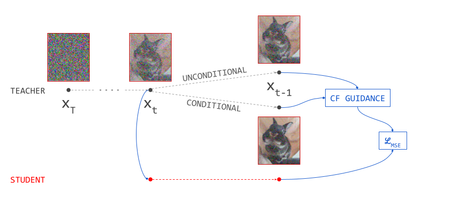
Guidance

I won’t repeat here how classifier-free guidance (CFG) works, as I have already written two blog posts about it, but modern diffusion sampling almost always relies heavily on this trick. Naturally, we might also want to use guidance with flow maps, but this is actually not straightforward.

Applying guidance during diffusion sampling involves modifying the denoiser prediction at each step using relatively simple linear operations. Because the modified prediction gets fed back into the denoiser model at the next step, the changes compound to have a highly complex and non-linear effect on the output of the sampling procedure. That makes this technique very powerful, despite its relative simplicity. It comes into conflict with distillation however, whose point is to dramatically reduce the number of sampling steps, which also reduces this compounding effect.

The easiest way to address this is to avoid applying guidance to the distilled model itself, and instead, apply it to the teacher model during distillation³⁹. The effect will then be incorporated and emulated by the student. This can be done in a few different ways: the simplest is to tune the guidance scale for the teacher and fix it during distillation, after which it cannot be changed. Instead of classifier-free guidance, other variants like autoguidance²⁵ can also be used in this way (as in e.g. AYF²¹).

A more advanced approach is to randomise the guidance scale, and feed the selected value into the student network as an extra conditioning signal (as in e.g. improved MeanFlow²⁰ and Terminal Velocity Matching¹⁷). The network then has to learn to incorporate the effect of guidance directly. This can be done both for distillation and for from-scratch training, using guidance-free training⁴⁰ (GFT).

Aside from helping to produce higher-quality samples, guidance also greatly simplifies the distribution that needs to be captured by the flow map. This is welcome, because flow maps are significantly more complex objects to model compared to denoisers. Simpler distributions are easier to model accurately with few steps.

Tricks of the trade

Flow map training dynamics can be quite chaotic due to the self-referential nature of consistency-based loss functions, but there are many other potential sources of instability as well, such as guidance-free training. All of the concrete implementations we have discussed come with a bag of tricks to reduce variance and help stabilise training. Exploring them all in detail would take us too far, but I would like to point out some general patterns:

• Initialisation: most approaches initialise the weights of the flow map model using the weights of a denoiser. In a distillation setting, this can be a copy of the teacher weights. An alternative approach is consistency mid-training⁴¹ (CMT), which is supposed to help bridge the gap between predicting infinitesimal steps (as a denoiser does) and larger finite steps.

• Output parameterisation: we have already discussed in section 1.3 that flow maps can be parameterised to predict the target position on the path (\(F\)), or the average velocity between the source and target position (\(V\)). Both of these can actually be challenging prediction targets for neural networks, as they are partially noisy. For diffusion models, it was recently suggested that parameterising the neural network to predict \(\hat{\mathbf{x}}_0\) is advantageous⁴², because data tends to live on a lower-dimensional nonlinear manifold within the high-dimensional output space, whereas isotropic noise (and therefore, noisy data) does not. Pixel MeanFlow³¹ extends this idea to flow maps, by parameterising the network to predict the ‘denoised image field’, which is a simple linear function of the average velocity and the current noisy input that is noise-free.

• Time step conditioning: unlike denoisers, which are conditioned on one time step, flow maps are conditioned on both a source and a target time step (except for some partial flow map variants, like consistency models). The simplest way to handle this is to have separate time step embeddings for both in the network. As an alternative, Decoupled MeanFlow²⁹ suggests partitioning the layers of the model, conditioning the earlier layers only on the source time step, and later layers only on the target time step. Yet another option is to condition the model on the difference between the time steps, i.e. the length of the interval. This is analogous to training a denoiser without any time step conditioning at all, which can work remarkably well in practice^{8 9}.

• Time step sampling and loss weighting: as with diffusion models, tweaking the time step sampling strategy during training is of paramount importance to ensure the model focuses its capacity on learning the right things. Since there are now two time steps to sample for each training example, these strategies can get quite complicated. Time-step dependent loss weighting is also very common, to account for the increased prediction difficulty as the time steps get farther apart, and to combat variance and balance gradient magnitudes. This is not surprising, given that training a flow map is essentially a massive multi-task learning problem. Since information propagates from small time step intervals to large ones, the \(s=t\) case is often significantly oversampled. When guidance is in play, guidance-dependent scaling is also common.

• Loss functions: sometimes, robust loss functions are used to reduce the impact of outliers (e.g. pseudo-Huber loss used in iCT³⁵), and perceptual loss functions are used to improve sample quality (e.g. LPIPS⁴³ used in CM¹¹, CTM³⁸ and PID²⁴).

• Curricula: since flow map training often boils down to fine-tuning a denoiser model in practice, various strategies have been developed to make this change in tasks less abrupt, and to help the model bootstrap its long-range predictions from shorter-range ones. This is can be implemented by gradually increasing the maximal distance between \(s\) and \(t\) over the course of training, for example. It is also common to train partial flow maps, which do not support making predictions for all possible pairs of \(s\) and \(t\) (e.g. FMM¹).

The landscape

To wrap up this section, here is a tabular overview of the methods we have discussed:

• The consistency rule on which each method is based is indicated by 🐶 (compositional), 🐱 (Lagrangian) or 🐔 (Eulerian).
• The learning setting is indicated by 🧑‍🏫 (distillation), 🪃 (from scratch, self-distillation) or 🌊 (from scratch, marginal-from-conditional learning).
• The output parameterisation is indicated by 🎯 (\(F\), target position on the path) or 🚀 (\(V\), average velocity). Note that sometimes, the loss is expressed in terms of \(F\) even when the network is parameterised to predict \(V\).
• JVP = Jacobian-vector product, SG = stop-gradient operation, FD = finite-difference approximation, aux = auxiliary denoiser.

An estimate of the cost of a single training iteration is also included in the table, using the ‘forward pass equivalent’ (FPE) metric. This assumes that a backward pass costs roughly twice as much as a forward pass (so run-of-the-mill neural network training has a cost of 3 FPE). We also assume that calculating a JVP and forward pass jointly costs twice as much as the forward pass alone, and calculating a backward pass through this combined operation costs 4 times as much. Needless to say, this is a rough approximation: in practice, some of these costs can be lower due to dead code elimination and other compiler optimisations, but also higher due to e.g. rematerialisation.

I have not included any additional costs caused by guidance (usually teacher guidance adds one extra FPE). Most methods with loss functions with multiple terms suggest using sub-batches for the different terms, and calculating the cheap terms more often, which can greatly reduce the effective cost in terms of FPE. For a fair comparison, I have not taken this into account, and assume that the full loss is calculated on the entire training batch.

It is incredibly easy to make mistakes when calculating these numbers, so I apologise for any inaccuracies (please feel free to point them out). Whether the computation graph is compiled (as with JAX or torch.compile) or not can also matter in practice. I have assumed that this is the case.

Applications and extensions

The obvious application of flow maps is faster sampling, but they have some other cool tricks up their sleeve. They can also be extended in interesting ways.

Faster sampling at scale

Terminal velocity matching¹⁷ has been applied to an image generation model with more than 10 billion parameters – all the more impressive, considering that it requires backpropagation through the JVP in the loss. Flow-anchored consistency models²⁷ were used to distill the 14B parameter Wan 2.2 video generation model on an image dataset, producing samples in 2-8 steps. Align Your Flow was used to distill the FLUX.1-dev image generation model and produce samples in 4 steps.

A slightly older success story is LCM-LoRA⁴⁴: low-rank adaptation (LoRA) modules for various variants of Stable Diffusion⁴⁵, which turn it from a diffusion model into a consistency model, enabling few-step sampling. Surprisingly, these modules are also able to work their magic on various fine-tuned versions of the original Stable Diffusion checkpoints, without modification.

In the audio domain, notable applications include ByteDance’s use of SplitMeanFlow³⁴ for their speech synthesis products, and Continuous Audio Language Models⁴⁶ (CALM), which have been applied to speech and music generation (samples of both are available here).

Efficient steering and post-training

Diffusion sampling is very malleable, with tweaks such as guidance proving highly effective in many applications. People have wanted to steer diffusion sampling based on arbitrary reward signals, but this is actually not straightforward: these signals are usually defined in terms of clean data, but during sampling, we only have noisy intermediate states. So by default, we can only really estimate rewards at the end of sampling. Unfortunately, by then, there is no more possibility for steering, so that defeats the point.

Reward-based steering requires an efficient way to look ahead at where the sample will end up. It should be differentiable, so that we can backpropagate reward signal gradients and use them to steer sampling. Several strategies have been explored for this:

• In some cases, the reward signal can be adapted so it is robust to noise, e.g. by training a classifier with noise augmentation to use for classifier guidance;
• Single-step diffusion sampling can be used, i.e. directly predicting \(\hat{\mathbf{x}}_0\) from the current noisy state \(\mathbf{x}_t\) in one pass^{47 48}. This is sometimes referred to as Tweedie’s formula. It is a fast and differentiable way to do look-ahead, but it produces blurry results. Most off-the-shelf models used to calculate reward signals are more robust to blurry inputs than to Gaussian noise, so this can still be a significant improvement.
• Sequential Monte Carlo⁴⁹ (SMC) involves drawing many samples in parallel. At each time step, trajectories with low reward scores (which can be evaluated using single-step diffusion sampling, for example) are removed, and trajectories with high scores are duplicated to replace them. This does not require backpropagating reward gradients, but it is quite expensive.

Flow maps offer an efficient differentiable look-ahead mechanism: instead of the blurry samples produced by single-step diffusion sampling, we can use ‘clean’ flow map samples to calculate the reward signal. Even if single-step sampling with flow maps is far from perfect, it will produce results that are much more in-distribution and less blurry than single-step diffusion sampling. Sabour et al. called this flow map trajectory tilting⁵⁰ (FMTT). Xu et al. also explored this idea for inverse problems⁵¹, and Woo et al. used it for protein design⁵².

Once we have a flow map that enables fast sampling, we could also just use it to draw many samples in parallel and filter them (SMC-style, but without look-ahead). This works remarkably well for some types of rewards, but for others, gradient-based steering provides superior results⁵⁰.

Although flow maps produce clean samples, they inevitably result in biased reward estimates when used for look-ahead. This is because an entire distribution of possible outcomes of the sampling process is represented by a single sample. It is not possible to draw multiple samples and average the reward across them, because flow maps are deterministic by design. Two workarounds have been explored for this:

• Variational Flow Maps⁵³ (VFM) use a ‘noise adapter’ trained based on a reward signal, to constrain the initial noise distribution used to sample from the flow map.
• Meta Flow Maps⁵⁴ and Diamond Maps⁵⁵ are stochastic flow maps, which are able to model the full posterior distribution from a given noisy intermediate state, while still enabling differentiable one-step sampling.

Aside from improved steering at inference time, these tweaks also enable reward-based post-training use cases, where being able to explore the reward landscape without mode collapse is important.

Discrete data

Some three years ago, I wrote about diffusion language models on this blog, pointing out that there are two main strategies to apply diffusion to categorical data: using a discrete corruption process (e.g. masking), or embedding discrete data in a continuous space, and using continuous diffusion instead. The emphasis in the research community has been on the former for the past few years, but recently, the latter approach is making a comeback.

Flow maps are playing a key role in this: as diffusion language models are gaining traction, people have been studying distillation methods extensively. It turns out that distilling discrete diffusion models down to very few steps hits a roadblock: independence assumptions between tokens in the sequence are unavoidable, and significantly deteriorate sample quality. Continuous methods do not have this issue, so there has been renewed interest as they are seen as more ‘distillable’.

In the first half of 2026, several works about training flow maps for categorical data have appeared on arXiv, including Categorical Flow Maps⁵⁶, Flow Map Language Models⁵⁷ and Discrete Flow Maps⁵⁸. All three demonstrate how to parameterise the flow map so that predictions are always constrained to the output space. This enables the use of the cross-entropy loss instead of the mean squared error for flow map training, which brings significant stability improvements. (This is the same idea as the ‘denoised image field’ parameterisation from pixel MeanFlow³¹, but applied here for a very different purpose.) Floor Eijkelboom recently published a really nice blog post about this revitalisation of continuous language diffusion research, which I had previously declared extinct after 2023.

On a personal note, I am quite excited about this, as my first and only diffusion paper to date was about Continuous Diffusion for Categorical Data⁵⁹ (CDCD). The motivation for that work was precisely to address some apparent shortcomings of discrete diffusion (like its inability to represent superpositions of possible outcomes in intermediate noisy states), and to tap into the rich existing toolbox for continous diffusion (guidance, efficient sampling, distillation), while sticking with familiar language modelling staples like Transformers and cross-entropy training. It is quite satisfying to see some of these advantages start to materialise!

Along with Categorical Flow Maps and Flow Map Language Models, we now have three separate papers heralding the triumphant return of continuous methods for language diffusion😶‍🌫️

Can you tell I'm excited?🫨https://t.co/SKS4OFtSG8https://t.co/kJ3cuFsggdhttps://t.co/aXXU4bUSMT https://t.co/oSCZkQ8rrH

— Sander Dieleman (@sedielem) April 26, 2026

Other extensions

Aside from discrete data, extensions to other non-Euclidean spaces (Riemannian manifolds) have been explored^{60 52}. This work is particularly relevant for scientific applications, where symmetries and curvature are commonly encountered. Another useful application is fast likelihood evaluation: diffusion models can be used to estimate likelihoods⁵, but the procedure is just as costly as sampling. The same flow map mechanism that speeds up sampling can be used to speed up this procedure as well^{61 62}.

Alternative strategies

Flow maps represent the trajectory-based approach to distilling diffusion models. For many applications, preserving the precise paths between noise and data is actually superfluous: the only thing we ultimately care about is to preserve the distribution at the data side, \(p(\mathbf{x}_0)\). Distributional distillation methods lean into this by relaxing the trajectory-preserving constraint. They minimise the distance between the generated distribution and the target distribution using score-based methods (Distribution Matching Distillation⁶³, Score Identity Distillation⁶⁴), statistical moments (Moment Matching Distillation⁶⁵, Inductive Moment Matching⁶⁶), adversaries (Adversarial Diffusion Distillation⁶⁷, Continuous Adversarial Flow Models⁶⁸), or the model’s own density estimates (Self-E⁶⁹).

Not having to preserve precise trajectories gives the student model more freedom to achieve its goal, which often produces very high-quality results in the few-step regime. This comes at the cost of giving up the smooth topology of the bijection between noise and data, the ability to estimate likelihoods, and the ability to map inputs from data to noise, which is useful for image editing and interpolation.

Some methods don’t fit neatly in either category: a middle ground option is to use Reflow¹⁰ to straighten the paths, instead of giving up on the bijection completely. We also previously discussed FreeFlow²², which combines a trajectory-based Lagrangian consistency approach with a distributional auxiliary denoiser strategy.

A very recent addition in the distributional camp is FD-loss⁷⁰, which suggests directly fine-tuning flow maps and diffusion models with a Fréchet distance metric as the loss function. Metrics like Fréchet Inception Distance (FID)⁷¹ have been used for evaluation of generative models for a long time, in spite of their perceived shortcomings. Using them as loss functions is difficult, because they require very large batch sizes. They work around that by backpropagating only through a smaller sub-batch (similar to BatchRenorm⁷²). I think the most surprising result is that this can be applied directly to standard diffusion models to turn them into great one-step generators.

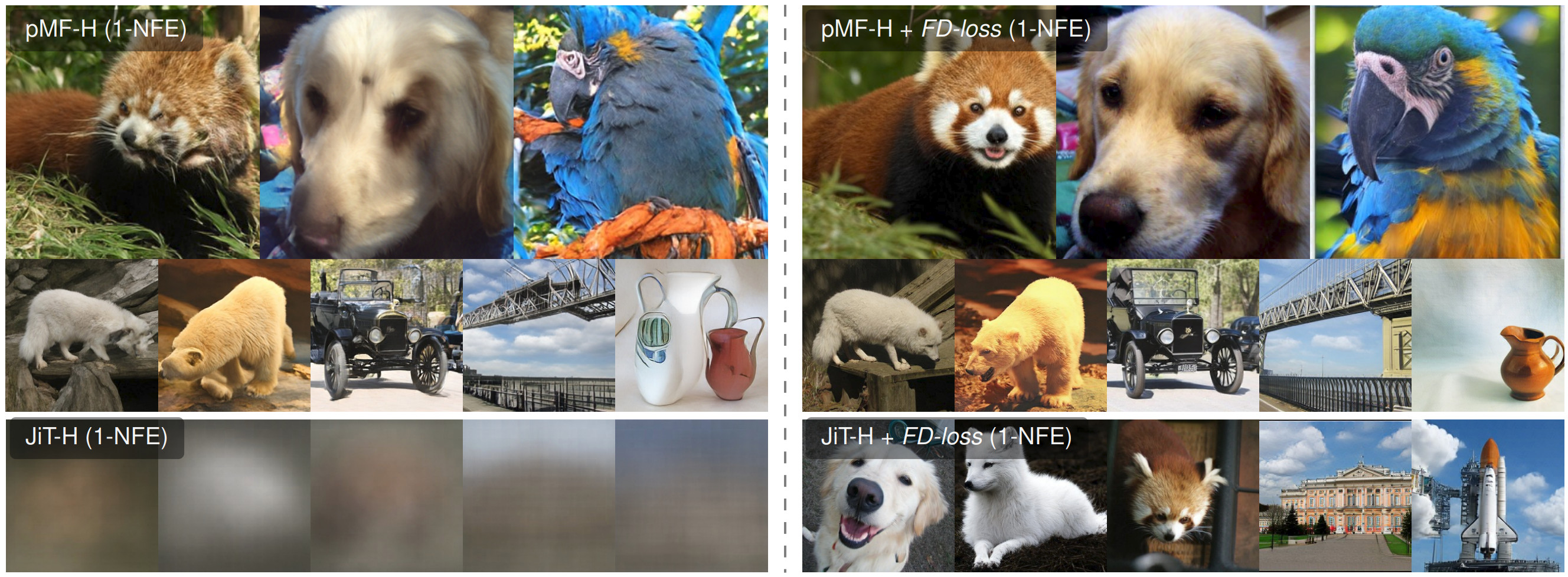
Pi-flow⁷³ suggests another strategy to speed up diffusion sampling: rather than learning to integrate the ODE or using a distributional approach, sampling steps are decoupled from denoiser evaluations. Rather than predicting a velocity, the network predicts a ‘network-free’ policy (e.g. a Gaussian mixture model), which can be used to predict velocities cheaply. This enables sampling with many steps but very few network evaluations.

Drifting models⁷⁴ mustered quite a bit of excitement recently, with a strategy for training one-step models that is conceptually related to diffusion, but quite different from it in practice: the distribution modelled by a feed-forward generator is evolved over the course of training using a ‘drifting field’ that pulls samples towards the data distribution. Personally, I am somewhat skeptical about the scalability of this approach, because it relies heavily on a good pre-trained feature space to work at all. Ivan Skorokhodov posted a great take about this work on Twitter.

Closing thoughts

First of all, thanks for sticking with me (and the animals 🐶🐔🐱) to the end! I hope this post provided a useful framework for recognising and understanding the relationships between various flow map methods, the consistency rules they are based on, and the tools at our disposal to make them practical and efficient. I hope I’ve also given you an idea of the possibilities they unlock.

Flow maps are not a silver bullet: their reliance on bootstrapping from denoisers (whether explicit, as in distillation, or implicit) already suggests that they get less reliable as the time interval we jump across increases. We are still calculating integrals after all – we are just precomputing them at training time (in an amortised way), instead of during sampling!

That said, with mature methods like improved MeanFlow (iMF) and Terminal Velocity Matching (TVM), promising applications to non-Euclidean and discrete data, and recent improvements to reward-based steering and fine-tuning, it certainly feels like we have come a long way towards making flow maps practically useful. What’s your flow map training recipe of choice? Please share your thoughts in the comments!

Disclosure regarding the use of AI in producing this blog post: I want to write in my own voice, and I want to respect everyone who takes the time to read what I write. Therefore, you will not find any passages or sentences in this post that are fully AI-generated. (Even the em dashes are all mine!) That said, I do occasionally consult AI when considering a particular turn of phrase, or to help me find the best wording (like a souped-up version of thesaurus.com). I primarily use it to help me understand papers and the relationship between them, and sometimes to create images and diagrams. AI was extensively used in the making of this blog post, but the prose is entirely ‘artisanal intelligence’. That is the level of AI involvement I am currently comfortable with.

If you would like to cite this post in an academic context, you can use this BibTeX snippet:

@misc{dieleman2026flowmaps,
  author = {Dieleman, Sander},
  title = {Learning the integral of a diffusion model},
  url = {https://sander.ai/2026/05/06/flow-maps.html},
  year = {2026}
}

Acknowledgements

Thanks to Bundle the bunny for modelling, and to kipply for permission to use this photograph. Thanks to my colleagues at Google DeepMind and to various members of the research community, whom I have discussed these topics with over the past year. Thanks especially to James Thornton, Valentin De Bortoli, Nicholas Boffi, Michael Albergo, Karsten Kreis and Xin Yu.

References

Generative models that make use of latent representations are everywhere nowadays, so I thought it was high time to dedicate a blog post to them. In what follows, I will talk at length about latents as a plural noun, which is the usual shorthand for latent representation. This terminology originated in the concept of latent variables in statistics, but it is worth noting that the meaning has drifted somewhat in this context. These latents do not represent any known underlying physical quantity which we cannot measure directly; rather, they capture perceptually meaningful information in a compact way, and in many cases they are a deterministic nonlinear function of the input signal (i.e. not random variables).

In what follows, I will assume a basic understanding of neural networks, generative models and related concepts. Below is an overview of the different sections of this post. Click to jump directly to a particular section.

1. The recipe
2. How we got here
3. Why two stages?
4. Trading off reconstruction quality and modelability
5. Controlling capacity
6. Curating and shaping the latent space
7. The tyranny of the grid
8. Latents for other modalities
9. Will end-to-end win in the end?
10. Closing thoughts
11. Acknowledgements
12. References

The recipe

The usual process for training a generative model in latent space consists of two stages:

1. Train an autoencoder on the input signals. This is a neural network consisting of two subnetworks, an encoder and a decoder. The former maps an input signal to its corresponding latent representation (encoding). The latter maps the latent representation back to the input domain (decoding).
2. Train a generative model on the latent representations. This involves taking the encoder from the first stage, and using it to extract latents for the training data. The generative model is then trained directly on these latents. Nowadays, this is usually either an autoregressive model or a diffusion model.

Once the autoencoder is trained in the first stage, its parameters will not change any further in the second stage: gradients from the second stage of the learning process are not backpropagated into the encoder. Another way to say this is that the encoder parameters are frozen in the second stage.

Note that the decoder part of the autoencoder plays no role in the second stage of training, but we will need it when sampling from the generative model, as that will generate outputs in latent space. The decoder enables us to map the generated latents back to the original input space.

Below is a diagram illustrating this two-stage training recipe. Networks whose parameters are learnt in the respective stages are indicated with a \(\nabla\) symbol, because this is almost always done using gradient-based learning. Networks whose parameters are frozen are indicated with a snowflake.

Several different loss functions are involved in the two training stages, which are indicated in red on the diagram:

• To ensure the encoder and decoder are able to convert input representations to latents and back with high fidelity, several loss functions constrain the reconstruction (decoder output) with respect to the input. These usualy include a simple regression loss, a perceptual loss and an adversarial loss.
• To constrain the capacity of the latents, an additional loss function is often applied directly to them during training, although this is not always the case. We will refer to this as the bottleneck loss, because the latent representation forms a bottleneck in the autoencoder network.
• In the second stage, the generative model is trained using its own loss function, separate from those used during the first stage. This is often the negative log-likelihood loss (for autoregressive models), or a diffusion loss.

Taking a closer look at the reconstruction-based losses, we have:

• the regression loss, which is sometimes the mean absolute error (MAE) measured in the input space (e.g. on pixels), but more often the mean squared error (MSE).
• the perceptual loss, which can take many forms, but more often than not, it makes use of another frozen pre-trained neural network to extract perceptual features. The loss encourages these features to match between the reconstruction and the input, which results in better preservation of high-frequency content that is largely ignored by the regression loss. LPIPS¹ is a popular choice for images.
• the adversarial loss, which uses a discriminator network which is co-trained with the autoencoder, as in generative adversarial networks (GANs)². The discriminator is trained to tell apart real input signals from reconstructions, and the autoencoder is trained to fool the discriminator into making mistakes. The goal is to improve the realism of the output, even if it means deviating further from the input signal. It is quite common for the adversarial loss to be disabled for some time at the start of training, to avoid instability.

Below is a more elaborate diagram of the first training stage, explicitly showing the other networks which typically play a role in this process.

It goes without saying that this generic recipe is often deviated from in one or more ways, especially for audio and video, but I have tried to summarise the most common ingredients found in most modern practical applications of this modelling approach.

How we got here

The two dominant generative modelling paradigms of today, autoregression and diffusion, were both initially applied to “raw” digital representations of perceptual signals, by which I mean pixels and waveforms. PixelRNN³ and PixelCNN⁴ generated images one pixel at a time. WaveNet⁵ and SampleRNN⁶ did the same for audio, producing waveform amplitudes one sample at a time. On the diffusion side, the original works that introduced⁷ and established^{8 9} the modelling paradigm all operated on pixels to produce images, and early works like WaveGrad¹⁰ and DiffWave¹¹ generated waveforms to produce sound.

However, it became clear very quickly that this strategy makes scaling up quite challenging. The most important reason for this can be summarised as follows: perceptual signals mostly consist of imperceptible noise. Or, to put it a different way: out of the total information content of a given signal, only a small fraction actually affects our perception of it. Therefore, it pays to ensure that our generative model can use its capacity efficiently, and focus on modelling just that fraction. That way, we can use smaller, faster and cheaper generative models without compromising on perceptual quality.

Latent autoregression

Autoregressive models of images took a huge leap forward with the seminal VQ-VAE paper¹². It suggested a practical strategy for learning discrete representations with neural networks, by inserting a vector quantisation bottleneck layer into an autoencoder. To learn such discrete latents for images, a convolutional encoder with several downsampling stages produced a spatial grid of vectors with a 4× lower resolution than the input (along both height and width, so 16× fewer spatial positions), and these vectors were then quantised by the bottleneck layer.

Now, we could generate images with PixelCNN-style models one latent vector at a time, rather than having to do it pixel by pixel. This significantly reduced the number of autoregressive sampling steps required, but perhaps more importantly, measuring the likelihood loss in the latent space rather than pixel space helped avoid wasting capacity on imperceptible noise. This is effectively a different loss function, putting more weight on perceptually relevant signal content, because a lot of the perceptually irrelevant signal content is not present in the latent vectors (see my blog post on typicality for more on this topic). The paper showed 128×128 generated images from a model trained on ImageNet, a resolution that had only been attainable with GANs² up to that point.

The discretisation was critical to its success, because autoregressive models were known to work much better with discrete inputs at the time. But perhaps even more importantly, the spatial structure of the latents allowed existing pixel-based models to be adapted very easily. Before this, VAEs (variational autoencoders^{13 14}) would typically compress an entire image into a single latent vector, resulting in a representation without any kind of topological structure. The grid structure of modern latent representations, which mirrors that of the “raw” input representation, is exploited in the network architecture of generative models to increase efficiency (through e.g. convolutions, recurrence or attention layers).

VQ-VAE 2¹⁵ further increased the resolution to 256x256 and dramatically improved image quality through scale, as well as the use of multiple levels of latent grids, structured in a hierarchy. This was followed by VQGAN¹⁶, which combined the adversarial learning mechanism of GANs with the VQ-VAE architecture. This enabled a dramatic increase of the resolution reduction factor from 4× to 16× (256× fewer spatial positions compared to pixel input), while still allowing for sharp and realistic reconstructions. The adversarial loss played a big role in this, encouraging realistic decoder output even when it is not possible to closely adhere to the original input signal.

VQGAN became a core technology enabling the rapid progress in generative modelling of perceptual signals that we’ve witnessed in the last five years. Its impact cannot be overestimated – I’ve gone as far as to say that it’s probably the main reason why GANs deserved to win the Test of Time award at NeurIPS 2024. The “assist” that the VQGAN paper provided, kept GANs relevant even after they were all but replaced by diffusion models for the base task of media generation.

IMO VQGAN is why GANs deserve the NeurIPS test of time award. Suddenly our image representations were an order of magnitude more compact. Absolute game changer for generative modelling at scale, and the basis for latent diffusion models.https://t.co/Ochh17IvGx

— Sander Dieleman (@sedielem) November 28, 2024

It is also worth pointing out just how much of the recipe from the previous section was conceived in this paper. The iterative generator isn’t usually autoregressive these days (Parti¹⁷, xAI’s recent Aurora model and, apparently, OpenAI’s GPT-4o are notable exceptions), and the quantisation bottleneck has been replaced, but everything else is still there. Especially the combination of a simple regression loss, a perceptual loss and an adversarial loss has stubbornly persisted, in spite of its apparent complexity. This kind of endurance is rare in a fast-moving field like machine learning – perhaps rivalled only by that of the largely unchanged Transformer architecture¹⁸ and the Adam optimiser¹⁹!

(While discrete representations played an essential role in making latent autoregression work at scale, I wanted to point out that autoregression in continuous space has also been made to work well recently^{20 21}.)

Latent diffusion

With latent autoregression gaining ground in the late 2010s, and diffusion models breaking through in the early 2020s, combining the strengths of both approaches was a natural next step. As with many ideas whose time has come, we saw a string of concurrent papers exploring this topic hit arXiv around the same time, in the second half of 2021^{22 23 24 25 26}. The most well-known of these is Rombach et al.’s High-Resolution Image Synthesis with Latent Diffusion Models²⁶, who reused their previous VQGAN work¹⁶ and swapped out the autoregressive Transformer for a UNet-based diffusion model. This formed the basis for the Stable Diffusion models. Other works explored similar ideas, albeit at a smaller scale²⁴, or for modalities other than images²².

It took a little bit of time for the approach to become mainstream. Early commercial text-to-image models made use of so-called resolution cascades, consisting of a base diffusion model that generates low-resolution images directly in pixel space, and one or more upsampling diffusion models that produce higher-resolution outputs conditioned on lower-resolution inputs. Examples include DALL-E 2 and Imagen 2. After Stable Diffusion, most moved to a latent-based approach (including DALL-E 3 and Imagen 3).

An important difference between autoregressive and diffusion models is the loss function used to train them. In the autoregressive case, things are relatively simple: you just maximise the likelihood (although other things have been tried as well²⁷). For diffusion, things are a little more interesting: the loss is an expectation over all noise levels, and the relative weighting of these noise levels significantly affects what the model learns (for an explanation of this, see my previous blog post on noise schedules, as well as my blog post about casting diffusion as autoregression in frequency space). This justifies an interpretation of the typical diffusion loss as a kind of perceptual loss function, which puts more emphasis on signal content that is more perceptually salient.

At first glance, this makes the two-stage approach seem redundant, as it operates in a similar way, i.e. filtering out perceptually irrelevant signal content, to avoid wasting model capacity on it. If we can rely on the diffusion loss to focus only on what matters perceptually, why do we need a separate representation learning stage to filter out the stuff that doesn’t? These two mechanisms turn out to be quite complementary in practice however, for two reasons:

• The way perception works at small and large scales, especially in the visual domain, seems to be fundamentally different – to the extent that modelling texture and fine-grained detail merits separate treatment, and an adversarial approach can be more suitable for this. I will discuss this in more detail in the next section.
• Training large, powerful diffusion models is inherently computationally intensive, and operating in a more compact latent space allows us to avoid having to work with bulky input representations. This helps to reduce memory requirements and speeds up training and sampling.

Some early works did consider an end-to-end approach, jointly learning the latent representation and the diffusion prior^{23 25}, but this didn’t really catch on. Although avoiding sequential dependencies between multiple stages of training is desirable from a practical perspective, the perceptual and computational benefits make it worth the hassle.

Why two stages?

As discussed before, it is important to ensure that generative models of perceptual signals can use their capacity efficiently, as this makes them much more cost-effective. This is essentially what the two-stage approach accomplishes: by extracting a more compact representation that focuses on the perceptually relevant fraction of signal content, and modelling that instead of the original representation, we are able to make relatively modestly sized generative models punch above their weight.

The fact that most bits of information in perceptual signals don’t actually matter perceptually is hardly a new observation: it is also the key idea underlying lossy compression, which enables us to store and transmit these signals at a fraction of the cost. Compression algorithms like JPEG and MP3 exploit the redundancies present in signals, as well as the fact that our audiovisual senses are more sensitive to low frequencies than to high frequencies, to represent perceptual signals with far fewer bits. (There are other perceptual effects that play a role, such as auditory masking for example, but non-uniform frequency sensitivity is the most important one.)

So why don’t we use these lossy compression techniques as a basis for our generative models then? This is not a bad idea, and several works have used these algorithms, or parts of them, for this purpose^{28 29 30}. But a very natural reflex for people working on generative models is to try to solve the problem with more machine learning, to see if we can do better than these “handcrafted” algorithms.

It’s not just hubris on the part of ML researchers, though: there is actually a very good reason to use learned latents, instead of using these pre-existing compressed representations. Unlike in the compression setting, where smaller is better, and size is all that matters, the goal of generative modelling also imposes other constraints: some representations are easier to model than others. It is crucial that some structure remains in the representation, which we can then exploit by endowing the generative model with the appropriate inductive biases. This requirement creates a trade-off between reconstruction quality and modelability of the latents, which we will investigate in the next section.

An important reason behind the efficacy of latent representations is how they lean in to the fact that our perception works differently at different scales. In the audio domain, this is readily apparent: very rapid changes in amplitude result in the perception of pitch, whereas changes on coarser time scales (e.g. drum beats) can be individually discerned. Less well-known is that the same phenomenon also plays an important role in visual perception: rapid local fluctuations in colour and intensity are perceived as textures. A while back, I tried to explain this on Twitter, and I will paraphrase that explanation here:

Because of the dramatic improvements in efficiency that the two-stage approach offers, we seem to be happy to put up with the additional complexity it entails – at least, for now. This increased efficiency results in faster and cheaper training runs, but perhaps more importantly, it can greatly accelerate sampling as well. With generative models that perform iterative refinement, this significant cost reduction is of course very welcome, because many forward passes through the model are required to produce a single sample.

Trading off reconstruction quality and modelability

The difference between lossy compression and latent representation learning is worth exploring in more detail. One can use machine learning for both, although most lossy compression algorithms in widespread use today do not. These algorithms are typically rooted in rate-distortion theory, which formalises and quantifies the relationship between the degree to which we are able to compress a signal (rate), and how much we allow the decompressed signal to deviate from the original (distortion).

For latent representation learning, we can extend this trade-off by introducing the concept of modelability or learnability, which characterises how challenging it is for generative models to capture the distribution of this representation. This results in a three-way rate-distortion-modelability trade-off, which is closely related to the rate-distortion-usefulness trade-off discussed by Tschannen et al. in the context of representation learning³¹. (Another popular way to extend this trade-off in a machine learning context is the rate-distortion-perception trade-off³², which explicitly distinguishes reconstruction fidelity from perceptual quality. To avoid overcomplicating things, I will not make this distinction here, instead treating distortion as a quantity measured in a perceptual space, rather than input space.)

It’s not immediately obvious why this is even a trade-off at all – why is modelability at odds with distortion? To understand this, consider how lossy compression algorithms operate: they take advantage of known signal structure to reduce redundancy. In the process, this structure is often removed from the compressed representation, because the decompression algorithm is able to reconstitute it. But structure in input signals is also exploited extensively in modern generative models, in the form of architectural inductive biases for example, which take advantage of signal properties like translation equivariance or specific characteristics of the frequency spectrum.

If we have an amazing algorithm that efficiently removes almost all redundancies from our input signals, we are making it very difficult for generative models to capture the unstructured variability that remains in the compressed signals. That is completely fine if compression is all we are after, but not if we want to do generative modelling. So we have to strike a balance: a good latent representation learning algorithm will detect and remove some redundancy, but keep some signal structure as well, so there is something left for the generative model to work with.

A good example of what not to do in this setting is entropy coding, which is actually a lossless compression method, but is also used as the final stage in many lossy schemes (e.g. Huffman coding in JPEG/PNG, or arithmetic coding in H.265). Entropy coding algorithms reduce redundancy by assigning shorter representations to frequently occurring patterns. This doesn’t remove any information at all, but it destroys structure. As a result, small changes in input signals could lead to much larger changes in the corresponding compressed signals, potentially making entropy-coded sequences considerably more difficult to model.

In contrast, latent representations tend to preserve a lot of signal structure. The figure below shows a few visualisations of Stable Diffusion latents for images (taken from the EQ-VAE paper³³). It is pretty easy to identify the animals just from visually inspecting the latents. They basically look like noisy, low-resolution images with distorted colours. This is why I like to think of image latents as merely “advanced pixels”, capturing a little bit of extra information that regular pixels wouldn’t, but mostly still behaving like pixels nonetheless.

It is safe to say that these latents are quite low-level. Whereas traditional VAEs would compress an entire image into a single feature vector, often resulting in a high-level representation that enables semantic manipulation³⁴, modern latent representations used for generative modelling of images are actually much closer to the pixel level. They are much higher-capacity, inheriting the grid structure of the input (though at a lower resolution). Each latent vector in the grid may abstract away some low-level image features such as textures, but it does not capture the semantics of the image content. This is also why most autoencoders do not make use of any additional conditioning signals such as text captions, as those mainly constrain high-level structure (though exceptions exist³⁵).

Controlling capacity

Two key design parameters control the capacity of a grid-structured latent space: the downsampling factor and the number of channels of the representation. If the latent representation is discrete, the codebook size is also important, as it imposes a hard limit on the number of bits information that the latents can contain. (Aside from these, regularisation strategies play an important role, but we will discuss their impact in the next section.)

As an example, an encoder might take a 256×256 pixel image as input, and produce a 32×32 grid of continuous latent vectors with 8 channels. This could be achieved using a stack of strided convolutions, or perhaps using a vision Transformer (ViT)³⁶ with patch size 8. The downsampling factor reduces the dimensionality along both width and height, so there are 64 times fewer latent vectors than pixels – but each latent vector has 8 components, while each pixel has only 3 (RGB). In aggregate, the latent representation is a tensor with \(\frac{w_{in} \cdot h_{in} \cdot c_{in}}{w_{out} \cdot h_{out} \cdot c_{out}} = \frac{256 \cdot 256 \cdot 3}{32 \cdot 32 \cdot 8} = 24\) times fewer components (i.e. floating point numbers) than the tensor representing the original image. I like to refer to this number as the tensor size reduction factor (TSR), to avoid confusion with spatial or temporal downsampling factors.

If we were to increase the downsampling factor of the encoder by 2×, the latent grid size would then be 16×16, and we could increase the channel count by 4× to 32 channels, to maintain the same TSR. There are usually a few different configurations for a given TSR that perform roughly equally in terms of reconstruction quality, especially in the case of video, where we can separately control the temporal and spatial downsampling factors. If we change the TSR, however (by changing the downsampling factor without changing the channel count, or vice versa), this usually has a profound impact on both reconstruction quality and modelability.

From a purely mathematical perspective, this is surprising: if the latents are real-valued, the size of the grid and the number of channels shouldn’t matter, because the information capacity of a single number is already infinite (neatly demonstrated by Tupper’s self-referential formula). But of course, there are several practical limitations that restrict the amount of information a single component of the latent representation is able to carry:

• we use floating point representations of real numbers, which have finite precision;
• in many formulations, the encoder adds some amount of noise, which further limits effective precision;
• neural networks aren’t very good at learning highly nonlinear functions of their input.

The first one is obvious: if you represent a number with 32 bits (single precision), that is also the maximal number of bits of information it can possibly convey. Adding noise further reduces the number of usable bits, because some of the low-order digits will be overpowered by it.

The last limitation is actually the more restrictive one, but it is less well understood: isn’t the entire point of neural networks to learn nonlinear functions? That is true, but they are naturally biased towards learning relatively simple functions³⁷. This is usually a feature, not a bug, because it increases the probability of learning a function that generalises to unseen data. But if we are trying to compress a lot of information into a few numbers, that will likely require a high degree of nonlinearity. There are some ways to assist neural networks with learning more nonlinear functions (such as Fourier features³⁸), but in our setting, highly nonlinear mappings will actually negatively affect modelability: they obfuscate signal structure, so this is not a good solution. Representations with more components offer a better trade-off.

The same applies to discrete latent representations: the discretisation imposes a hard limit on the information content of the representation, but whether that capacity can be used efficiently depends chiefly on how expressive the encoder is, and how well the quantisation strategy works in practice (i.e. whether it achieves a high level of codebook utilisation by using the different codes as evenly as possible). I believe the most commonly used approach today is still the original VQ bottleneck from VQ-VAE¹², but a recent improvement which provides better gradient estimates using a “rotation trick”³⁹ seems promising in terms of codebook utilisation and end-to-end performance. Some alternatives without explicitly learnt codebooks have also gained traction recently: finite scalar quantisation (FSQ)⁴⁰, lookup-free quantisation (LFQ)⁴¹ and binary spherical quantisation (BSQ)⁴².

To recap, choosing the right TSR is key: a larger latent representation will yield better reconstruction quality (higher rate, lower distortion), but may negatively affect modelability. With a larger representation, there are simply more bits of information to model, therefore requiring more capacity in the generative model. In practice, this trade-off is usually tuned empirically. This can be an expensive affair, because there aren’t really any reliable proxy metrics for modelability that are cheap to compute. Therefore, it requires repeatedly training large enough generative models to get meaningful results.

Hansen-Estruch et al.⁴³ recently shared an extensive exploration of latent space capacity and the various factors that influence it (their key findings are clearly highlighted within the text). There is currently a trend toward increasing the spatial downsampling factor, and maintaining the TSR by also increasing the number of channels accordingly, in order to facilitate image and video generation at higher resolutions (e.g. 32× in LTX-Video⁴⁴ and GAIA-2⁴⁵, up to 64× in DCAE⁴⁶).

Curating and shaping the latent space

So far, we have talked about the capacity of latent representations, i.e. how many bits of information should go in them. It is just as important to control precisely which bits from the original input signals should be preserved in the latents, and how this information is presented. I will refer to the former as curating the latent space, and to the latter as shaping the latent space – the distinction is subtle, but important. Many regularisation strategies have been devised to shape, curate and control the capacity of latents. I will focus on the continuous case, but many of the same considerations apply to discrete latents as well.

VQGAN and KL-regularised latents

Rombach et al.²⁶ suggested two regularisation strategies for continuous latent spaces:

• Follow the original VQGAN recipe, reinterpreting the quantisation step as part of the decoder, rather than the encoder, to get a continuous representation (VQ-reg);
• Remove the quantisation step from the VQGAN recipe altogether, and replace it with a KL penalty, as in regular VAEs (KL-reg).

The idea of making only minimal changes to VQGAN to produce continuous latents (for use with diffusion models) is clever: the setup worked well for autoregressive models, and the quantisation during training serves as a safeguard to ensure that the latents don’t end up encoding too much information. However, as we discussed previously, this probably isn’t really necessary in most cases, because encoder expressivity is usually the limiting factor.

KL regularisation, on the other hand, is a core part of the traditional VAE setup: it is one of the two terms constituting the evidence lower bound (ELBO), which bounds the likelihood from below and enables VAE training to tractably (but indirectly) maximise the likelihood of the data. It encourages the latents to follow the imposed prior distribution (usually Gaussian). Crucially however, the ELBO is only truly a lower bound on the likelihood if there is no scaling hyperparameter in front of this term. Yet almost invariably, the KL term used to regularise continuous latent spaces is scaled down significantly (usually by several orders of magnitude), all but severing the connection with the variational inference context in which it originally arose.

The reason is simple: an unscaled KL term has too strong an effect, imposing a stringent limit on latent capacity and thus severely degrading reconstruction quality. The pragmatic response to that is naturally to scale down its relative contribution to the training loss. (Aside: in settings where one cares less about reconstruction quality, and more about semantic interpretability and disentanglement of the learnt representation, increasing the scale of the KL term can also be fruitful, as in beta-VAE³⁴.)

We are veering firmly into opinion territory here, but I feel there is currently quite a bit of magical thinking around the effect of the KL term. It is often suggested that this term encourages the latents to follow a Gaussian distribution, but with the scale factors that are typically used, this effect is way too weak to be meaningful. Even for “proper” VAEs, the aggregate posterior is rarely actually Gaussian^{47 48}.

All of this renders the “V” in “VAE” basically meaningless, in my opinion – its relevance is largely historical. We may as well drop it and talk about KL-regularised autoencoders instead, which more accurately reflects modern practice. The most important effect of the KL term in this setting is to supress outliers and constrain the scale of the latents to some extent. In other words: while the KL term is often presented as constraining capacity, the way it is used in practice mainly constrains the shape of the latents (but even that effect is relatively modest).

Tweaking reconstruction losses

The usual trio of reconstruction losses (regression, perceptual and adversarial) clearly plays an important role in maximising the quality of decoded signals, but it is also worth studying how these losses impact the latents, specifically in terms of curation (i.e. which information they learn to encode). As discussed in section 3, a good latent space in the visual domain makes abstraction of texture to some degree. How do these losses help achieve that?

A useful thought experiment is to consider what happens when we drop the perceptual and adversarial losses, retaining only the regression loss, as in traditional VAEs. This will tend to result in blurry reconstructions. Regression losses do not favour any particular kind of signal content by design, so in the case of images, they will focus on low-frequency content, simply because there is more of it. In natural images, the power of different spatial frequencies tends to be proportional to their inverse square – the higher the frequency, the less power (see my previous blog post for an illustrated analysis of this phenomenon). Since high frequencies constitute only a tiny fraction of the total signal power, the regression loss more strongly rewards accurate prediction of low frequencies than high ones. The relative perceptual importance of these high frequencies is much larger than the fraction of total signal power they represent, and blurry looking reconstructions are the well-known result.

Since texture is primarily composed of precisely these high frequencies which the regression loss largely ignores, we end up with a latent space that doesn’t make abstraction of texture, but rather erases textural information altogether. From a perceptual standpoint, that is a particularly undesirable form of latent space curation. This demonstrates the importance of the other two reconstruction loss terms, which ensure that the latents can encode some textural information.

If the regression loss has these undesirable properties, which require other loss terms to mitigate, perhaps we could drop it altogether? It turns out that’s not a great idea either, because the perceptual and adversarial losses are much harder to optimise and tend to have pathological local minima (they are usually based on pre-trained neural networks, after all). The regression loss acts as a sort of regulariser, continually providing guardrails against ending up in the bad parts of parameter space as training progresses.

Many strategies using different flavours of reconstruction losses have been suggested, and I won’t cover this space exhaustively, but here are a few examples from the literature, to give you an idea of the variety:

• The aforementioned DCAE⁴⁶ does not deviate too far from the original VQGAN recipe, only replacing the L2 regression loss (MSE) with L1 (MAE). It keeps the LPIPS perceptual loss and the PatchGAN⁴⁹ discriminator. It does however use multiple stages of training, with the adversarial loss only enabled in the last stage.
• ViT-VQGAN⁵⁰ combines two regression losses, the L2 loss and the logit-Laplace loss⁵¹, and uses the StyleGAN⁵² discriminator as well as the LPIPS perceptual loss.
• LTX-Video⁴⁴ introduces a video-aware loss based on the discrete wavelet transform (DWT), and uses a modified strategy for the adversarial loss which they call reconstruction-GAN.

As with many classic dishes, every chef still has their own recipe!

Representation learning vs. reconstruction

The design choices we have discussed so far usually impact not just reconstruction quality, but also the kind of latent space that is learnt. The reconstruction losses in particular do double duty: they ensure high-quality decoder output, and play an important role in curating the latent space as well. This raises the question whether it is actually desirable to kill two birds with one stone, as we have been doing. I would argue that the answer is no.

Learning a good compact representation for generative modelling on the one hand, and learning to decode that representation back to the input space on the other hand, are two separate tasks. Modern autoencoders are expected to learn to do both at once. The fact that this works reasonably well in practice is certainly a welcome convenience: training an autoencoder is already stage one of a two-stage training process, so ideally we wouldn’t want to complicate it any further (although having multiple autoencoder training stages is not unheard of^{46 53}). But this setup also needlessly conflates the two tasks, and some choices that are optimal for one task might not be for the other.

My colleagues and I actually made this point in a latent generative modelling paper⁵⁴, all the way back in 2019 (I recently tweeted about it as well). When the decoder is autoregressive, conflating the two tasks is particularly problematic, so we suggested using a separate non-autoregressive auxiliary decoder to provide the learning signal for the encoder. The main decoder is prevented from influencing the latent representation at all, by not backpropagating its gradients through to the encoder. It is therefore fully focused on maximising reconstruction quality, while the auxiliary decoder takes care of shaping and curating the latent space. All parts of the autoencoder can still be trained jointly, so the additional complexity is limited. The auxiliary decoder does of course increase the cost of training, but it can be discarded afterwards.

Although the idea of using autoregressive decoders in pixel space, as we did for that paper, has not aged well at all (to put it mildly), I believe using auxiliary decoders to separate the representation learning and reconstruction tasks is still a very relevant idea today. An auxiliary decoder that optimises a different loss, or that has a different architecture (or both), could provide a better learning signal for representation learning and result in better generative modelling performance.

Zhu et al.⁵⁵ recently came to the same conclusion (see section 2.1 of their paper), and constructed a discrete latent representation using K-means on DINOv2⁵⁶ features, combined with a separately trained decoder. Reusing representations learnt with self-supervised learning for generative modelling has historically been more common for audio models^{57 58 59 60} – perhaps because audio practitioners are already accustomed to the idea of training vocoders that turn predetermined intermediate representations (e.g. mel-spectrograms) back into audio waveforms.

Regularising for modelability

Shaping, curating and constraining the capacity of latents can all affect their modelability:

• Capacity constraints determine how much information is in the latents. The higher the capacity, the more powerful the generative model will have to be to adequately capture all of the information they contain.
• Shaping can be important to enable efficient modelling. The same information can be represented in many different ways, and some are easier to model than others. Scaling and standardisation are important to get right (especially for diffusion models), but higher-order statistics and correlation structure also matter.
• Curation influences modelability, because some kinds of information are much easier to model than others. If the latents encode information about unpredictable noise in the input signal, that will make them less predictable as well. Here’s an interesting tweet that demonstrates how this affects the Stable Diffusion XL VAE⁶¹:

The sdxl-VAE models a substantial amount of noise. Things we can't even see. It meticulously encodes the noise, uses precious bottleneck capacity to store it, then faithfully reconstructs it in the decoder.

I grabbed what I thought was a simple black vector circle on a white… pic.twitter.com/eK7ZtLJ6lc

— Rudy Gilman (@rgilman33) April 14, 2025

Here, I want to make the connection to the idea of \(\mathcal{V}\)-information, proposed by Xu et al.⁶², which extends the concept of mutual information to account for computational constraints (h/t @jxmnop on Twitter for bringing this work to my attention). In other words, the usability of information varies depending on how computationally challenging it is for an observer to discern, and we can try to quantify this. If a piece of information requires a powerful neural net to extract, the \(\mathcal{V}\)-information in the input is lower than in the case where a simple linear probe suffices – even when the absolute information content measured in bits is identical. Clearly, maximising the \(\mathcal{V}\)-information of the latent representation is desirable, in order to minimise the computational requirements for the generative model to be able to make sense of it. The rate-distortion-usefulness trade-off described by Tschannen et al., which I mentioned before³¹, supports the same conclusion.

As discussed earlier, the KL penalty probably doesn’t do quite as much to Gaussianise or otherwise smoothen the latent space as many seem to believe. So what can we do instead to make the latents easier to model?

• Use generative priors: co-train a (lightweight) latent generative model with the autoencoder, and make the latents easy to model by backpropagating the generative loss into the encoder, as in LARP⁶³ or CRT⁶⁴. This requires careful tuning of loss weights, because the generative loss and the reconstruction losses are at odds with each other: latents are easiest to model when they encode no information at all!

• Supervise with pre-trained representations: encourage the latents to be predictive of existing high-quality representations (e.g. DINOv2⁵⁶ features), as in VA-VAE⁶⁵, MAETok⁶⁶ or GigaTok⁶⁷.

• Encourage equivariance: make it so that certain transformations of the input (e.g. rescaling, rotations) produce corresponding latent representations that are transformed similarly, as in AuraEquiVAE, EQ-VAE³³ and AF-VAE⁶⁸. The figure from the EQ-VAE paper that I used in section 4 shows the profound impact that this constraint can have on the spatial smoothness of the latent space. Skorokhodov et al.⁶⁹ came to the same conclusion based on spectral analysis of latent spaces: equivariance regularisation makes the latent spectrum more similar to that of the pixel space inputs, which improves modelability.

This was just a small sample of possible regularisation strategies, all of which attempt to increase the \(\mathcal{V}\)-information of the latents in one way or another. This list is very far from exhaustive, both in terms of the strategies themselves and the works cited, so I encourage you to share any other relevant work you’ve come across in the comments!

Diffusion all the way down

A specific class of autoencoders for learning latent representations deserves a closer look: those with diffusion decoders. While a more typical decoder architecture features a feedforward network that directly outputs pixel values in one forward pass, and is trained adversarially, an alternative that’s gaining popularity is to use diffusion for the task of latent decoding (as well as for modelling the distribution of the latents). This impacts reconstruction quality, but it also affects what kind of representation is learnt.

SWYCC⁷⁰, \(\epsilon\)-VAE⁷¹ and DiTo⁷² are some recent works that explore this approach. They motivate this in a few different ways:

• latents learnt with diffusion decoders provide a more principled, theoretically grounded way of doing hierarchical generative modelling;
• they can be trained with just the MSE loss, which simplifies things and improves robustness (adversarial losses are pretty finicky to tune, after all);
• applying the principle of iterative refinement to decoding improves output quality.

I can’t really argue with any of these points, but I do want to point out one significant weakness of diffusion decoders: their computational cost, and the effect this has on decoder latency. I believe one of the key reasons that most commercially deployed diffusion models today are latent models, is that compact latent representations help us avoid iterative refinement in input space, which is slow and costly. Performing the iterative sampling procedure in latent space, and then going back to input space with a single forward pass at the end, is significantly faster.

With that in mind, reintroducing input-space iterative refinement for the decoding task looks to me like it largely defeats the point of the two-stage approach. If we are going to be paying that cost, we might as well opt for something like simple diffusion^{73 74} to scale up single-stage generative models instead.

Not so fast, you might say – can’t we use one of the many diffusion distillation methods to bring down the number of steps required? In a setting such as this one, with a very rich conditioning signal (i.e. the latent representation), these methods have indeed proven effective even down to the single-step sampling regime: the stronger the conditioning, the fewer steps are needed for high quality distillation results.

DALL-E 3’s consistency decoder⁷⁵ is a great practical example of this: they reused the Stable Diffusion²⁶ latent space and trained a new diffusion-based decoder, which was then distilled down to just two sampling steps using consistency distillation⁷⁶. While it is still more costly than the original adversarial decoder in terms of latency, the visual fidelity of the outputs is significantly improved.

Music2Latent⁷⁷ is another example of this approach, operating on spectrogram representations of music audio. Their autoencoder with a consistency decoder is trained end-to-end (unlike DALL-E 3’s, which reuses a pre-trained encoder), and is able to produce high-fidelity outputs in a single step. This means decoding once again requires only a single forward pass, as it does for adversarial decoders.

FlowMo⁵³ is an autoencoder with a diffusion decoder that uses a post-training stage to encourage mode-seeking behaviour. As mentioned before, for the task of decoding latent representations, dropping modes and focusing on realism over diversity is actually desirable, because it requires less model capacity and does not negatively impact perceptual quality. Adversarial losses tend to result in mode dropping, but diffusion-based losses do not. This two-stage training strategy enables the diffusion decoder to mimic this behaviour – although a significant number of sampling steps are still required, so the computational cost is considerably higher than for a typical adversarial decoder.

Some earlier works on diffusion autoencoders, such as Diff-AE⁷⁸ and DiffuseVAE⁷⁹, are more focused on learning high-level semantic representations in the vein of old-school VAEs, without topological structure, and with a focus on controllability and disentanglement. DisCo-Diff⁸⁰ sits somewhere in between, augmenting a diffusion model with a sequence of discrete latents, which can be modelled by an autoregressive prior.

Removing the need for adversarial training would certainly simplify things, so diffusion autoencoders are an interesting (and recently, quite popular) field of study in that regard. Still, it seems challenging to compete with adversarial decoders when it comes to latency, so I don’t think we are quite ready to abandon them. I very much look forward to an updated recipe that doesn’t require adversarial training, yet matches the current crop of adversarial decoders in terms of both visual quality and latency!

The tyranny of the grid

Digital representations of perceptual modalities are usually grid-structured, because they arise as uniformly sampled (and quantised) versions of the underlying physical signals. Images give rise to 2D grids of pixels, videos to 3D grids, and audio signals to 1D grids (i.e. sequences). The uniform sampling implies that there is a fixed quantum (i.e. distance or amount of time) between adjacent grid positions.

Perceptual signals also tend to be approximately stationary in time and space in a statistical sense. Combined with uniform sampling, this results in a rich topological structure, which we gratefully take advantage of when designing neural network architectures to process them: we use extensive weight sharing to benefit from invariance and equivariance properties, implemented through convolutions, recurrence and attention mechanisms.

Without a doubt, our ability to exploit this structure is one of the key reasons why we have been able to build machine learning models that are as powerful as they are. A corollary of this is that preserving this structure when designing latent spaces is a great idea. Our most powerful neural network designs architecturally depend on it, because they were originally built to process these digital signals directly. They will be better at processing latent representations instead, if those representations have the same kind of structure.

It also offers significant benefits for the autoencoders which learn to produce the latents: because of the stationarity, and because they only need to learn about local signal structure, they can be trained on smaller crops or segments of input signals. If we impose the right architectural constraints (limiting the receptive field of each position in the encoder and the decoder), they will generalise out of the box to larger grids than they were trained on. This has the potential to greatly reduce the training cost for the first stage.

It’s not all sunshine and rainbows though: we have discussed how perceptual signals are highly redundant, and unfortunately, this redundancy is unevenly distributed. Some parts of the signal might contain lots of detail that is perceptually salient, where others are almost devoid of information. In the image of a dog in a field that we used previously, consider a 100×100 pixel patch centered on the dog’s head, and then compare that to a 100×100 pixel patch in the top right corner of the image, which contains only the blue sky.

If we construct a latent representation which inherits the 2D grid structure of the input, and use it to encode this image, we will necessarily use the exact same amount of capacity to encode both of these patches. If we make the representation rich enough to capture all the relevant perceptual detail for the dog’s head, we will waste a lot of capacity to encode a similar-sized patch of sky. In other words, preserving the grid structure comes at a significant cost to the efficiency of the latent representation.

This is what I call the tyranny of the grid: our ability to process grid-structured data with neural networks is highly developed, and deviating from this structure adds complexity and makes the modelling task considerably harder and less hardware-friendly, so we generally don’t do this. But in terms of encoding efficiency, this is actually quite wasteful, because of the non-uniform distribution of perceptually salient information in audiovisual signals.

The Transformer architecture is actually relatively well-positioned to bolster a rebellion against this tyranny: while we often think of it as a sequence model, it is actually designed to process set-valued data, and any additional topological structure that relates elements of a set to each other is expressed through positional encoding. This makes deviating from a regular grid structure more practical than it is for convolutional or recurrent architectures. (Several years ago, my colleagues and I explored this idea for speech generation using variable-rate discrete representations⁸¹.)

Relaxing the topology of the latent space in the context of two-stage generative modelling appears to be gaining some traction lately:

• TiTok⁸² and FlowMo⁵³ learn sequence-structured latents from images, reducing the grid dimensionality from 2D to 1D. The development of large language models has given us extremely powerful sequence models, so this is a reasonable kind of structure to aim for.
• One-D-Piece⁸³, FlexTok⁸⁴ and Semanticist⁸⁵ do the same, but use a nested dropout mechanism⁸⁶ to induce a coarse-to-fine structure in the latent sequence. This in turn enables the sequence length to be adapted to the complexity of each individual input image, and to the level of detail required in the reconstruction. A few other mechanisms for adaptive 1D tokenisation have been proposed, e.g. ElasticTok⁸⁷ and ALIT⁸⁸. CAT⁸⁹ also explores this kind of adaptivity, but still maintains a 2D grid structure and only adapts its resolution.
• TokenSet⁹⁰ goes a step further and uses an autoencoder that produces “bags of tokens”, abandoning the grid completely.

Aside from CAT, all of these have in common that they learn latent spaces that are considerably more semantically high-level than the ones we have mostly been talking about so far. In terms of abstraction level, they probably sit somewhere in the middle between “advanced pixels” and the vector-valued latents of old-school VAEs. In fact, FlexTok and Semanticist’s 1D sequence encoders expect low-level latents from an existing 2D grid-structured encoder as input, literally building an additional abstraction level on top of a pre-existing low-level latent space. TiTok and One-D-Piece also make use of an existing 2D grid-structured latent space as part of a multi-stage training approach. A related idea is to reuse the language domain as a high-level latent representation for images⁹¹.

In the discrete setting, some work has investigated whether commonly occurring patterns of tokens in a grid can be combined into larger sub-units, using ideas from language tokenisation: DiscreTalk⁹² is an early example in the speech domain, using SentencePiece⁹³ on top of VQ tokens. Zhang et al.’s BPE Image Tokenizer⁹⁴ is a more recent incarnation of this idea, using an enhanced byte-pair encoding⁹⁵ algorithm on VQGAN tokens.

Latents for other modalities

We have chiefly focused on the visual domain so far, only briefly mentioning audio in some places. This is because learning latents for images is something we have gotten pretty good at, and image generation with the two-stage approach has been extensively studied (and productionised!) in recent years. We have a well-developed body of research on perceptual losses, and a host of discriminator architectures that enable adversarial training to focus on perceptually relevant image content.

With video, we remain in the visual domain, but a temporal dimension is introduced, which presents some challenges. One could simply reuse image latents and extract them frame-by-frame to get a latent video representation, but this would likely lead to temporal artifacts (like flickering). More importantly, it does not allow for taking advantage of temporal redundancy. I believe our tools for spatiotemporal latent representation learning are considerably less well developed, and how to account for the human perception of motion to improve efficiency is less well understood for now. This is in spite of the fact that video compression algorithms all make use of motion estimation to improve efficiency.

The same goes for audio: while there has been significant adoption of the two-stage recipe^{96 97 98}, there seems to be considerably less of a broad consensus on the necessary modifications to make it work for this modality. As mentioned before, for audio it is also much more common to reuse representations learnt with self-supervised learning.

What about language? This is not a perceptual modality, but maybe the two-stage approach could improve the efficiency of large language models as well? This is not straightforward, as it turns out. Language is inherently much less compressible than perceptual signals: it developed as a means of efficient communication, so there is considerably less redundancy. Which is not to say there isn’t any: Shannon famously estimated English to be 50% redundant⁹⁹. But recall that images, audio and video can be compressed by several orders of magnitude with relatively minimal perceptual distortion, which is not possible with language without losing nuance or important semantic information.

Tokenisers used for language models tend to be lossless (e.g. BPE⁹⁵, SentencePiece⁹³), so the resulting tokens aren’t usually viewed as “latents” (Byte Latent Transformer¹⁰⁰ does use this framing for its dynamic tokenisation strategy, however). The relative lack of redundancy in language has not stopped people from trying to learn lossy higher-level representations, though! The techniques used for perceptual signals may not carry over, but several other methods to learn representations at the sentence or paragraph level have been explored^{101 102 103}.

Will end-to-end win in the end?

When deep learning rose to prominence, the dominant narrative was that we would replace handcrafted features with end-to-end learning wherever possible. Jointly learning all processing stages would allow these stages to co-adapt and cooperate to maximise performance, while also simplifying things from an engineering perspective. This is more or less what ended up happening in computer vision and speech processing. In that light, it is rather ironic that the dominant generative modelling paradigm for perceptual signals today is a two-stage approach. Both stages tend to be learnt, but it’s not exactly end-to-end!

Text-to-image, text-to-video and text-to-audio models deployed in products today are, for the most part, using intermediate latent representations. It is worth pondering whether this is a temporary status quo, or likely to continue to be the case. Two-stage training does introduce a significant amount of complexity after all, and apart from being more elegant, end-to-end learning would help ensure that all parts of a system are perfectly in tune with a single, overarching objective.

As discussed, iterative refinement in the input space is slow and costly, and I think this is likely to remain the case for a while longer – especially as we continue to ramp up the quality, resolution and/or length of the generated signals. The benefits of latents for training efficiency and sampling latency are not something we are likely to be happy to give up on, and there are currently no viable alternatives that have been demonstrated to work at scale. This is somewhat of a contentious point, because some researchers seem to believe the time has come to move towards an end-to-end approach. Personally, I think it’s too early.

So, when will we be ready to move back to single-stage generative models? Methods like simple diffusion^{73 74}, Ambient Space Flow Transformers¹⁰⁴ and PixelFlow¹⁰⁵ have shown that this already works pretty well, even at relatively high resolutions – it just isn’t very cost-effective yet. But hardware keeps getting better and faster at an incredible rate, so I suspect we will eventually reach a point where the relative inefficiency of input-space models starts to be economically preferable over the increased engineering complexity of latent-space models. When exactly this will happen depends on the modality, the rate of hardware improvements and research progress, so I will stop short of making a concrete prediction.

It used to be the case that we needed latents to ensure that generative models would focus on learning about perceptually relevant signal content, while ignoring entropy that is not visually salient. Recall that the likelihood loss in input space is particularly bad at this, and switching to measuring likelihood in latent space dramatically improved results obtained with likelihood-based models¹². Arguably, this is no longer the case, because we have figured out how to perceptually re-weight the likelihood loss function for both autoregressive and diffusion models^{106 107}, removing an important obstacle to scaling. But in spite of that, the computational efficiency benefits of latent-space models remain as relevant as ever.

A third alternative, which I’ve only briefly mentioned so far, is the resolution cascade approach. This requires no representation learning, but still splits up the generative modelling problem into multiple stages. Some early commercial models used this approach, but it seems to have fallen out of favour. I believe this is because the division of labour between the different stages is suboptimal – upsampling models have to do too much of the work, and this makes them more prone to error accumulation across stages.

Closing thoughts

To wrap up, here are some key takeaways:

• Latents for generative modelling are usually quite unlike VAE latents from way back when: it makes more sense to think of them as advanced pixels than as high-level semantic representations.
• Having two stages enables us to have different loss functions for each, and significantly improves computational efficiency by avoiding iterative sampling in the input space.
• Latents add complexity, but the computational efficiency benefits are large enough for us to tolerate this complexity – at least for now.
• Three main aspects to consider when designing latent spaces are capacity (how many bits of information are encoded in the latents), curation (which bits from the input signals are retained) and shape (how this information is presented).
• Preserving structure (i.e. topology, statistics) in the latent space is important to make it easy to model, even if this is sometimes worse from an efficiency perspective.
• The V in VAE is vestigial: the autoencoders used in two-stage latent generative models are really KL-regularised AEs, and usually barely regularised at that.
• The combination of a regression loss, a perceptual loss and an adversarial loss is surprisingly entrenched. Almost all modern implementations of autoencoders for latent representation learning are variations on this theme.
• Representation learning and reconstruction are two separate tasks, and while it is convenient to do both at once, this might not be optimal.

Several years ago, I wrote on this blog that representation learning has an important role to play in generative modelling. Though it wasn’t exactly prophetic at the time (VQ-VAE had already existed for three years), the focus in the representation learning community back then was firmly on high-level semantic representations that are useful for discriminative tasks. It was a lot more common to hear about generative modelling in service of representation learning, than vice versa. How the tables have turned! The arrival of VQGAN¹⁶ a few months later was probably what cemented the path we now find ourselves on, and made two-stage generative modelling go mainstream.

Thank you for reading what ended up being my longest blog post yet! I’m keen to hear your thoughts here in the comments, on Twitter (yes, that’s what I’m calling it), or on BlueSky.

If you would like to cite this post in an academic context, you can use this BibTeX snippet:

@misc{dieleman2025latents,
  author = {Dieleman, Sander},
  title = {Generative modelling in latent space},
  url = {https://sander.ai/2025/04/15/latents.html},
  year = {2025}
}

Acknowledgements

Thanks to my colleagues at Google DeepMind for various discussions, which continue to shape my thoughts on this topic! Thanks also to Stefan Baumann, Rami Seid, Charles Foster, Ethan Smith, Simo Ryu, Theodoros Kouzelis and Jack Gallagher.

References

This blog post is also available as a Python notebook in Google Colab , with the code used to produce all the plots and animations.

Last year, I wrote a blog post describing various different perspectives on diffusion. The idea was to highlight a number of connections between diffusion models and other classes of models and concepts. In recent months, I have given a few talks where I discussed some of these perspectives. My talk at the EEML 2024 summer school in Novi Sad, Serbia, was recorded and is available on YouTube. Based on the response I got from this talk, the link between diffusion models and autoregressive models seems to be particularly thought-provoking. That’s why I figured it could be useful to explore this a bit further.

In this blog post, I will unpack the above claim, and try to make it obvious that this is the case, at least for visual data. To make things more tangible, I decided to write this entire blog post in the form of a Python notebook (using Google Colab). That way, you can easily reproduce the plots and analyses yourself, and modify them to observe what happens. I hope this format will also help drive home the point that this connection between diffusion models and autoregressive models is “real”, and not just a theoretical idealisation that doesn’t hold up in practice.

In what follows, I will assume a basic understanding of diffusion models and the core concepts behind them. If you’ve watched the talk I linked above, you should be able to follow along. Alternatively, the perspectives on diffusion blog post should also suffice as preparatory reading. Some knowledge of the Fourier transform will also be helpful.

Below is an overview of the different sections of this post. Click to jump directly to a particular section.

1. Two forms of iterative refinement
2. A spectral view of diffusion
3. What about sound?
4. Unstable equilibrium
5. Closing thoughts
6. Acknowledgements
7. References

Two forms of iterative refinement

Autoregression and diffusion are currently the two dominant generative modelling paradigms. There are many more ways to build generative models: flow-based models and adversarial models are just two possible alternatives (I discussed a few more in an earlier blog post).

Both autoregression and diffusion differ from most of these alternatives, by splitting up the difficult task of generating data from complex distributions into smaller subtasks that are easier to learn. Autoregression does this by casting the data to be modelled into the shape of a sequence, and recursively predicting one sequence element at a time. Diffusion instead works by defining a corruption process that gradually destroys all structure in the data, and training a model to learn to invert this process step by step.

This iterative refinement approach to generative modelling is very powerful, because it allows us to construct very deep computational graphs for generation, without having to backpropagate through them during training. Indeed, both autoregressive models and diffusion models learn to perform a single step of refinement at a time – the generative process is not trained end-to-end. It is only when we try to sample from the model that we connect all these steps together, by sequentially performing the subtasks: predicting one sequence element after another in the case of autoregression, or gradually denoising the input step-by-step in the case of diffusion.

Because this underlying iterative approach is common to both paradigms, people have often sought to connect the two. One could frame autoregression as a special case of discrete diffusion, for example, with a corruption process that gradually replaces tokens by “mask tokens” from right to left, eventually ending up with a fully masked sequence. In the next few sections, we will do the opposite, framing diffusion as a special case of autoregression, albeit approximate.

Today, most language models are autoregressive, while most models of images and video are diffusion-based. In many other application domains (e.g. protein design, planning in reinforcement learning, …), diffusion models are also becoming more prevalent. I think this dichotomy, which can be summarised as “autoregression for language, and diffusion for everything else”, is quite interesting. I have written about it before, and I will have more to say about it in a later section of this post.

A spectral view of diffusion

Image spectra

When diffusion models rose to prominence for image generation, people noticed quite quickly that they tend to produce images in a coarse-to-fine manner. The large-scale structure present in the image seems to be decided in earlier denoising steps, whereas later denoising steps add more and more fine-grained details.

To formalise this observation, we can use signal processing, and more specifically spectral analysis. By decomposing an image into its constituent spatial frequency components, we can more precisely tease apart its coarse- and fine-grained structure, which correspond to low and high frequencies respectively.

We can use the 2D Fourier transform to obtain a frequency representation of an image. This representation is invertible, i.e. it contains the same information as the pixel representation – it is just organised in a different way. Like the pixel representation, it is a 2D grid-structured object, with the same width and height as the original image, but the axes now correspond to horizontal and vertical spatial frequencies, rather than spatial positions.

To see what this looks like, let’s take some images and visualise their spectra.

Shown above on the first row are four images from the Imagenette dataset, a subset of the ImageNet dataset (I picked it because it is relatively fast to load).

The Fourier transform is typically complex-valued, so the next two rows visualise the magnitude and the phase of the spectrum respectively. Because the magnitude varies greatly across different frequencies, its logarithm is shown. The phase is an angle, which varies between \(-\pi\) and \(\pi\). Note that we only calculate the spectrum for the green colour channel – we could calculate it for the other two channels as well, but they would look very similar.

The centre of the spectrum corresponds to the lowest spatial frequencies, and the frequencies increase as we move outward to the edges. This allows us to see where most of the energy in the input signal is concentrated. Note that by default, it is the other way around (low frequencies in the corner, high frequencies in the middle), but np.fft.fftshift allows us to swap these, which yields a much nicer looking visualisation that makes the structure of the spectrum more apparent.

A lot of interesting things can be said about the phase structure of natural images, but in what follows, we will primarily focus on the magnitude spectrum. The square of the magnitude is the power, so in practice we often look at the power spectrum instead. Note that the logarithm of the power spectrum is simply that of the magnitude spectrum, multiplied by two.

Looking at the spectra, we now have a more formal way to reason about different feature scales in images, but that still doesn’t explain why diffusion models exhibit this coarse-to-fine behaviour. To see why this happens, we need to examine what a typical image spectrum looks like. To do this, we will make abstraction of the directional nature of frequencies in 2D space, simply by slicing the spectrum along a certain angle, rotating that slice all around, and then averaging the slices across all rotations. This yields a one-dimensional curve: the radially averaged power spectral density, or RAPSD.

Below is an animation that shows individual directional slices of the 2D spectrum on a log-log plot, which are averaged to obtain the RAPSD.

Let’s see what that looks like for the four images above. We will use the pysteps library, which comes with a handy function to calculate the RAPSD in one go.

The RAPSD is best visualised on a log-log plot, to account for the large variation in scale. We chop off the so-called DC component (with frequency 0) to avoid taking the logarithm of 0.

Another thing this visualisation makes apparent is that the curves are remarkably close to being straight lines. A straight line on a log-log plot implies that there might be a power law lurking behind all of this.

Indeed, this turns out to be the case: natural image spectra tend to approximately follow a power law, which means that the power \(P(f)\) of a particular frequency \(f\) is proportional to \(f^{-\alpha}\), where \(\alpha\) is a parameter^{1 2 3}. In practice, \(\alpha\) is often remarkably close to 2 (which corresponds to the spectrum of pink noise in two dimensions).

We can get closer to the “typical” RAPSD by taking the average across a bunch of images (in the log-domain).

As I’m sure you will agree, that is pretty unequivocally a power law!

To estimate the exponent \(\alpha\), we can simply use linear regression in log-log space. Before proceeding however, it is useful to resample our averaged RAPSD so the sample points are linearly spaced in log-log space – otherwise our fit will be dominated by the high frequencies, where we have many more sample points.

We obtain an estimate \(\hat{\alpha} = 2.454\), which is a bit higher than the typical value of 2. As far as I understand, this can be explained by the presence of man-made objects in many of the images we used, because they tend to have smooth surfaces and straight angles, which results in comparatively more low-frequency content and less high-frequency content compared to images of nature. Let’s see what our fit looks like.

Noisy image spectra

A crucial aspect of diffusion models is the corruption process, which involves adding Gaussian noise. Let’s see what this does to the spectrum. The first question to ask is: what does the spectrum of noise look like? We can repeat the previous procedure, but replace the image input with standard Gaussian noise. For contrast, we will visualise the spectrum of the noise alongside that of the images from before.

The RAPSD of Gaussian noise is also a straight line on a log-log plot; but a horizontal one, rather than one that slopes down. This reflects the fact that Gaussian noise contains all frequencies in equal measure. The Fourier transform of Gaussian noise is itself Gaussian noise, so its power must be equal across all frequencies in expectation.

When we add noise to the images and look at the spectrum of the resulting noisy images, we see a hinge shape:

Why does this happen? Recall that the Fourier transform is linear: the Fourier transform of the sum of two things, is the sum of the Fourier transforms of those things. Because the power of the different frequencies varies across orders of magnitude, one of the terms in this sum tends to drown out the other. This is what happens at low frequencies, where the image spectrum dominates, and hence the green curve overlaps with the red curve. At high frequencies on the other hand, the noise spectrum dominates, and the green curve overlaps with the blue curve. In between, there is a transition zone where the power of both spectra is roughly matched.

If we increase the variance of the noise by scaling the noise term, we increase its power, and as a result, its RAPSD will shift upward (which is also a consequence of the linearity of the Fourier transform). This means a smaller part of the image spectrum now juts out above the waterline: the increasing power of the noise looks like the rising tide!

At this point, I’d like to revisit a diagram from the perspectives on diffusion blog post, where I originally drew the connection between diffusion and autoregression in frequency space, which is shown below.

These idealised plots of the spectra of images, noise, and their superposition match up pretty well with the real versions. When I originally drew this, I didn’t actually realise just how closely this reflects reality!

What these plots reveal is an approximate equivalence (in expectation) between adding noise to images, and low-pass filtering them. The noise will drown out some portion of the high frequencies, and leave the low frequencies untouched. The variance of the noise determines the cut-off frequency of the filter. Note that this is the case only because of the characteristic shape of natural image spectra.

The animation below shows how the spectrum changes as we gradually add more noise, until it eventually overpowers all frequency components, and all image content is gone.

Diffusion

With this in mind, it becomes apparent that the corruption process used in diffusion models is actually gradually filtering out more and more high-frequency information from the input image, and the different time steps of the process correspond to a frequency decomposition: basically an approximate version of the Fourier transform!

Since diffusion models themselves are tasked with reversing this corruption process step-by-step, they end up roughly predicting the next higher frequency component at each step of the generative process, given all preceding (lower) frequency components. This is a soft version of autoregression in frequency space, or if you want to make it sound fancier, approximate spectral autoregression.

To the best of my knowledge, Rissanen et al. (2022)⁴ were the first to apply this kind of analysis to diffusion in the context of generative modelling (see §2.2 in the paper). Their work directly inspired this blog post.

In many popular formulations of diffusion, the corruption process does not just involve adding noise, but also rescaling the input to keep the total variance within a reasonable range (or constant, in the case of variance-preserving diffusion). I have largely ignored this so far, because it doesn’t materially change anything about the intuitive interpretation. Scaling the input simply results in the RAPSD shifting up or down a bit.

Which frequencies are modelled at which noise levels?

There seems to be a monotonic relationship between noise levels and spatial frequencies (and hence feature scales). Can we characterise this quantitatively?

We can try, but it is important to emphasise that this relationship is only really valid in expectation, averaged across many images: for individual images, the spectrum will not be a perfectly straight line, and it will not typically be monotonically decreasing.

Even if we ignore all that, the “elbow” of the hinge-shaped spectrum of a noisy image is not very sharp, so it is clear that there is quite a large transition zone where we cannot unequivocally say that a particular frequency is dominated by either signal or noise. So this is, at best, a very smooth approximation to the “hard” autoregression used in e.g. large language models.

Keeping all of that in mind, let us construct a mapping from noise levels to frequencies for a particular diffusion process and a particular image distribution, by choosing a signal-to-noise ratio (SNR) threshold, below which we will consider the signal to be undetectable. This choice is quite arbitrary, and we will just have to choose a value and stick with it. We can choose 1 to keep things simple, which means that we consider the signal to be detectable if its power is equal to or greater than the power of the noise.

Consider a Gaussian diffusion process for which \(\mathbf{x}_t = \alpha(t)\mathbf{x}_0 + \sigma(t) \mathbf{\varepsilon}\), with \(\mathbf{x}_0\) an example from the data distribution, and \(\mathbf{\varepsilon}\) standard Gaussian noise.

Let us define \(\mathcal{R}[\mathbf{x}](f)\) as the RAPSD of an image \(\mathbf{x}\) evaluated at frequency \(f\). We will call the SNR threshold \(\tau\). If we consider a particular time step \(t\), then assuming the RAPSD is monotonically decreasing, we can define the maximal detectable frequency \(f_\max\) at this time step in the process as the maximal value of \(f\) for which:

Recall that the Fourier transform is a linear operator, and \(\mathcal{R}\) is a radial average of the square of its magnitude. Therefore, scaling the input to \(\mathcal{R}\) by a real value means the output gets scaled by its square. We can use this to simplify things:

We can further simplify this by noting that \(\forall f: \mathcal{R}[\mathbf{\varepsilon}](f) = 1\):

To construct such a mapping in practice, we first have to choose a diffusion process, which gives us the functional form of \(\sigma(t)\) and \(\alpha(t)\). To keep things simple, we can use the rectified flow⁵ / flow matching⁶ process, as used in Stable Diffusion 3⁷, for which \(\sigma(t) = t\) and \(\alpha(t) = 1 - t\). Combined with \(\tau = 1\), this yields:

With these choices, we can now determine the shape of \(f_\max(t)\) and visualise it.

The frequencies here are relative: if the bandwidth of the signal is 1, then 0.5 corresponds to the Nyquist frequency, i.e. the maximal frequency that is representable with the given bandwidth.

Note that all representable frequencies are detectable at time steps near 0. As \(t\) increases, so does the noise level, and hence \(f_\max\) starts dropping, until it eventually reaches 0 (no detectable signal frequencies are left) close to \(t = 1\).

What about sound?

All of the analysis above hinges on the fact that spectra of natural images typically follow a power law. Diffusion models have also been used to generate audio^{8 9}, which is the other main perceptual modality besides the visual. A very natural question to ask is whether the same interpretation makes sense in the audio domain as well.

To establish that, we will grab a dataset of typical audio recordings that we might want to build a generative model of: speech and music.

Along with each audio player, a spectrogram is shown: this is a time-frequency representation of the sound, which is obtained by applying the Fourier transform to short overlapping windows of the waveform and stacking the resulting magnitude vectors together in a 2D matrix.

For the purpose of comparing the spectrum of sound with that of images, we will use the 1-dimensional analogue of the RAPSD, which is simply the squared magnitude of the 1D Fourier transform.

These are a lot noisier than the image spectra, which is not surprising as these are not averaged over directions, like the RAPSD is. But aside from that, they don’t really look like straight lines either – the power law shape is nowhere to be seen!

I won’t speculate about why images exhibit this behaviour and sound seemingly doesn’t, but it is certainly interesting (feel free to speculate away in the comments!). To get a cleaner view, we can again average the spectra of many clips in the log domain, as we did with the RAPSDs of images.

Definitely not a power law. More importantly, it is not monotonic, so adding progressively more Gaussian noise to this does not obfuscate frequencies in descending order: the “diffusion is just spectral autoregression” meme does not apply to audio waveforms!

The average spectrum of our dataset exhibits a peak around 300-400 Hz. This is not too far off the typical spectrum of green noise, which has more energy in the region of 500 Hz. Green noise is supposed to sound like “the background noise of the world”.

As the animation above shows, the different frequencies present in audio signals still get filtered out gradually from least powerful to most powerful, because the spectrum of Gaussian noise is still flat, just like in the image domain. But as the audio spectrum does not monotonically decay with increasing frequency, the order is not monotonic in terms of the frequencies themselves.

What does this mean for diffusion in the waveform domain? That’s not entirely clear to me. It certainly makes the link with autoregressive models weaker, but I’m not sure if there are any negative implications for generative modelling performance.

One observation that does perhaps indicate that this is the case, is that a lot of diffusion models of audio described in the literature do not operate directly in the waveform domain. It is quite common to first extract some form of spectrogram (as we did earlier), and perform diffusion in that space, essentially treating it like an image^{10 11 12}. Note that spectrograms are a somewhat lossy representation of sound, because phase information is typically discarded.

To understand the implications of this for diffusion models, we will extract log-scaled mel-spectrograms from the sound clips we have used before. The mel scale is a nonlinear frequency scale which is intended to be perceptually uniform, and which is very commonly used in spectral analysis of sound.

Next, we will interpret these spectrograms as images and look at their spectra. Taking the spectrum of a spectrum might seem odd – some of you might even suggest that it is pointless, because the Fourier transform is its own inverse! But note that there are a few nonlinear operations happening in between: taking the magnitude (discarding the phase information), mel-binning and log-scaling. As a result, this second Fourier transform doesn’t just undo the first one.

It seems like the power law has resurfaced! We can look at the average in the log-domain again to get a smoother curve.

I found this pretty surprising. I actually used to object quite strongly to the idea of treating spectrograms as images, as in this tweet in response to Riffusion, a variant of Stable Diffusion finetuned on spectrograms:

Me: "NOOO, you can't just treat spectrograms as images, the frequency and time axes have completely different semantics, there is no locality in frequency and ..."

These guys: "Stable diffusion go brrr" https://t.co/Akv8aZl8Rv

— Sander Dieleman (@sedielem) December 15, 2022

… but I have always had to concede that it seems to work pretty well in practice, and perhaps the fact that spectrograms exhibit power-law spectra is one reason why.

There is also an interesting link with mel-frequency cepstral coefficients (MFCCs), a popular feature representation for speech and music processing which predates the advent of deep learning. These features are constructed by taking the discrete cosine transform (DCT) of a mel-spectrogram. The resulting spectrum-of-a-spectrum is often referred to as the cepstrum.

So with this approach, perhaps the meme applies to sound after all, albeit with a slight adjustment: diffusion on spectrograms is just cepstral autoregression.

Unstable equilibrium

So far, we have talked about a spectral perspective on diffusion, but we have not really discussed how it can be used to explain why diffusion works so well for images. The fact that this interpretation is possible for images, but not for some other domains, does not automatically imply that the method should also work better.

However, it does mean that the diffusion loss, which is a weighted average across all noise levels, is also implicitly a weighted average over all spatial frequencies in the image domain. Being able to individually weight these frequencies in the loss according to their relative importance is key, because the sensitivity of the human visual system to particular frequencies varies greatly. This effectively makes the diffusion training objective a kind of perceptual loss, and I believe it largely explains the success of diffusion models in the visual domain (together with classifier-free guidance).

Going beyond images, one could use the same line of reasoning to try and understand why diffusion models haven’t really caught on in the domain of language modelling so far (I wrote more about this last year). The interpretation in terms of a frequency decomposition is not really applicable there, and hence being able to change the relative weighting of noise levels in the loss doesn’t quite have the same impact on the quality of generated outputs.

For language modelling, autoregression is currently the dominant modelling paradigm, and while diffusion-based approaches have been making inroads recently^{13 14 15}, a full-on takeover does not look like it is in the cards in the short term.

This results in the following status quo: we use autoregression for language, and we use diffusion for pretty much everything else. Of course, I realise that I have just been arguing that these two approaches are not all that different in spirit. But in practice, their implementations can look quite different, and a lot of knowledge and experience that practitioners have built up is specific to each paradigm.

To me, this feels like an unstable equilibrium, because the future is multimodal. We will ultimately want models that natively understand language, images, sound and other modalities mixed together. Grafting these two different modelling paradigms together to construct multimodal models is effective to some extent, and certainly interesting from a research perspective, but it brings with it an increased level of complexity (i.e. having to master two different modelling paradigms) which I don’t believe practitioners will tolerate in the long run.

So in the longer term, it seems plausible that we could go back to using autoregression across all modalities, perhaps borrowing some ideas from diffusion in the process^{16 17}. Alternatively, we might figure out how to build multimodal diffusion models for all modalities, including language. I don’t know which it is going to be, but both of those outcomes ultimately seem more likely than the current situation persisting.

One might ask, if diffusion is really just approximate autoregression in frequency space, why not just do exact autoregression in frequency space instead, and maybe that will work just as well? That would mean we can use autoregression across all modalities, and resolve the “instability” in one go. Nash et al. (2021)¹⁸, Tian et al. (2024)¹⁶ and Mattar et al. (2024)¹⁹ explore this direction.

There is a good reason not to take this shortcut, however: the diffusion sampling procedure is exceptionally flexible, in ways that autoregressive sampling is not. For example, the number of sampling steps can be chosen at test time (this isn’t impossible for autoregressive models, but it is much less straightforward to achieve). This flexibility also enables various distillation methods to reduce the number of steps required, and classifier-free guidance to improve sample quality. Before we do anything rash and ditch diffusion altogether, we will probably want to figure out a way to avoid having to give up some of these benefits.

Closing thoughts

When I first had a closer look at the spectra of real images myself, I realised that the link between diffusion models and autoregressive models is even stronger than I had originally thought – in the image domain, at least. This is ultimately why I decided to write this blog post in a notebook, to make it easier for others to see this for themselves as well. More broadly speaking, I find that learning by “doing” has a much more lasting effect than learning by reading, and hopefully making this post interactive can help with that.

There are of course many other ways to connect the two modelling paradigms of diffusion and autoregression, which I won’t go into here, but it is becoming a rather popular topic of inquiry^{20 21 22}.

If you enjoyed this post, I strongly recommend also reading Rissanen et al. (2022)’s paper on generative modelling with inverse heat dissipation⁴, which inspired it.

This blog-post-in-a-notebook was an experiment, so any feedback on the format is very welcome! It’s a bit more work, but hopefully some readers will derive some benefit from it. If there are enough of you, perhaps I will do more of these in the future. Please share your thoughts in the comments!

To wrap up, below are some low-effort memes I made when I should have been working on this blog post instead.

The interpretation of diffusion as autoregression in the frequency domain seems to be stirring up a lot of thought! (I may or may not have a new blog post in the works 🧐) pic.twitter.com/XSxP27pKSt

— Sander Dieleman (@sedielem) August 4, 2024

It's so much easier to tweet low-effort memes which assert that diffusion is just autoregression in frequency space, than it is to write a blog post about it 🤷 (but I'm doing both!) pic.twitter.com/snLQavtZBf

— Sander Dieleman (@sedielem) August 22, 2024

If you would like to cite this post in an academic context, you can use this BibTeX snippet:

@misc{dieleman2024spectral,
  author = {Dieleman, Sander},
  title = {Diffusion is spectral autoregression},
  url = {https://sander.ai/2024/09/02/spectral-autoregression.html},
  year = {2024}
}

Acknowledgements

Thanks to my colleagues at Google DeepMind for various discussions, which continue to shape my thoughts on this topic! In particular, thanks to Robert Riachi, Ruben Villegas and Daniel Zoran.

References

All of my blog posts are somewhat subjective, and I usually don’t shy away from highlighting my favourite ideas, formalisms and papers. That said, this one is probably a bit more opinionated still, maybe even a tad spicy! Probably the spiciest part is the title, but I promise I will explain my motivation for choosing it. At the same time, I also hope to provide some insight into the aspects of diffusion models that influence the relative importance of different noise levels, and why this matters.

This post will be most useful to readers familiar with the basics of diffusion models. If that’s not you, don’t worry; I have a whole series of blog posts with references to bring you up to speed! As a starting point, check out Diffusion models are autoencoders and Perspectives on diffusion. Over the past few years, I have written a few more on specific topics as well, such as guidance and distillation. A list of all my blog posts can be found here.

Below is an overview of the different sections of this post. Click to jump directly to a particular section.

1. Noise schedules: a whirlwind tour
2. Noise levels: focusing on what matters
3. Model design choices: what might tip the balance?
4. Noise schedules are a superfluous abstraction
5. Adaptive weighting mechanisms
6. Closing thoughts
7. Acknowledgements
8. References

Noise schedules: a whirlwind tour

Most descriptions of diffusion models consider a process that gradually corrupts examples of a data distribution with noise. The task of the model is then to learn how to undo the corruption. Additive Gaussian noise is most commonly used as the corruption method. This has the nice property that adding noise multiple times in sequence yields the same outcome (in a distributional sense) as adding noise once with a higher standard deviation. The total standard deviation is found as \(\sigma = \sqrt{ \sum_i \sigma_i^2}\), where \(\sigma_1, \sigma_2, \ldots\) are the standard deviations of the noise added at each point in the sequence.

Therefore, at each point in the corruption process, we can ask: what is the total amount of noise that has been added so far – what is its standard deviation? We can write this as \(\sigma(t)\), where \(t\) is a time variable that indicates how far the corruption process has progressed. This function \(\sigma(t)\) is what we typically refer to as the noise schedule. Another consequence of this property of Gaussian noise is that we can jump forward to any point in the corruption process in a single step, simply by adding noise with standard deviation \(\sigma(t)\) to a noiseless input example. The distribution of the result is exactly the same as if we had run the corruption process step by step.

In addition to adding noise, the original noiseless input is often rescaled by a time-dependent scale factor \(\alpha(t)\) to stop it from growing uncontrollably. Given an example \(\mathbf{x}_0\), we can turn it into a noisy example \(\mathbf{x}_t = \alpha(t) \mathbf{x}_0 + \sigma(t) \varepsilon\), where \(\varepsilon \sim \mathcal{N}(0, 1)\).

• The most popular formulation of diffusion models chooses \(\alpha(t) = \sqrt{1 - \sigma(t)^2}\), which also requires that \(\sigma(t) \leq 1\). This is because if we assume \(\mathrm{Var}[\mathbf{x}_0] = 1\), we can derive that \(\mathrm{Var}[\mathbf{x}_t] = 1\) for all \(t\). In other words, this choice is variance-preserving: the total variance (of the signal plus the added noise) is \(1\) at every step of the corruption process. In the literature, this is referred to as VP diffusion¹. While \(\mathrm{Var}[\mathbf{x}_0] = 1\) isn’t always true in practice (for example, image pixels scaled to \([-1, 1]\) will have a lower variance), it’s often close enough that things still work well in practice.

• An alternative is to do no rescaling at all, i.e. \(\alpha(t) = 1\). This is called variance-exploding or VE diffusion. It requires \(\sigma(t)\) to grow quite large to be able to drown out all of the signal for large values of \(t\), which is a prerequisite for diffusion models to work well. For image pixels scaled to \([-1, 1]\), we might want to ramp up \(\sigma(t)\) all the way to ~100 before it becomes more or less impossible to discern any remaining signal structure. The exact maximum value is a hyperparameter which depends on the data distribution. It was popularised by Karras et al. (2022)².

• More recently, formalisms based on flow matching³ and rectified flow⁴ have gained popularity. They set \(\alpha(t) = 1 - \sigma(t)\), which is also sometimes referred to as sub-VP diffusion. This is because in this case, \(\mathrm{Var}[\mathbf{x}_t] \leq 1\) when we assume \(\mathrm{Var}[\mathbf{x}_0] = 1\). This choice is supposed to result in straighter paths through input space between data and noise, which in turn reduces the number of sampling steps required to hit a certain level of quality (see my previous blog post for more about sampling with fewer steps). Stable Diffusion 3 uses this approach⁵.

By convention, \(t\) typically ranges from \(0\) to \(1\) in the VP and sub-VP settings, so that no noise is present at \(t=0\) (hence \(\sigma(0) = 0\) and \(\alpha(0) = 1\)), and at \(t=1\) the noise has completely drowned out the signal (hence \(\sigma(1) = 1\) and \(\alpha(1) = 0\)). In the flow matching literature, the direction of \(t\) is usually reversed, so that \(t=0\) corresponds to maximal noise and \(t=1\) to minimal noise instead, but I am sticking to the diffusion convention here. Note that \(t\) can be a continuous time variable, or a discrete index, depending on which paper you’re reading; here, we will assume it is continuous.

Let’s look at a few different noise schedules that have been used in the literature. It goes without saying that this is far from an exhaustive list – I will only mention some of the most popular and interesting options.

• The so-called linear schedule was proposed in the original DDPM paper⁶. This paper uses a discrete-time formulation, and specifies the schedule in terms of the variances of \(q(\mathbf{x}_{t+1} \mid \mathbf{x}_t)\) (corresponding to a single discrete step in the forward process), which they call \(\beta_t\). These variances increase linearly with \(t\), which is where the name comes from. In our formalism, this corresponds to \(\sigma(t) = \sqrt{1 - \prod_{i=1}^t (1 - \beta_i)}\), so while \(\beta_t\) might be a linear function of \(t\), \(\sigma(t)\) is not.

• The cosine schedule is arguably the most popular noise schedule to this day. It was introduced by Nichol & Dhariwal⁷ after observing that the linear schedule is suboptimal for high-resolution images, because it gets too noisy too quickly. This corresponds to \(\sigma(t) = \sin \left(\frac{t/T + s}{1 + s} \frac{\pi}{2} \right)\), where \(T\) is the maximal (discrete) time step, and \(s\) is an offset hyperparameter. It might seem like calling this the sine schedule would have been more appropriate, but the naming is again the result of using a slightly different formalism. (There is no standardised formalism for diffusion models, so every paper tends to describe things using different conventions and terminology, which is something I’ve written about before.)

• Karras et al. (2022)² use the variance-exploding formalism in combination with the simplest noise schedule you can imagine: \(\sigma(t) = t\). Because of this, they get rid of the “time” variable altogether, and express everything directly in terms of \(\sigma\) (because they are effectively equivalent). This is not the whole story however, and we’ll revisit this approach later.

• To adjust a pre-existing noise schedule to be more suitable for high-resolution images, both Chen (2023)⁸ and Hoogeboom et al. (2023)⁹ suggest “shifting” the schedule to account for the fact that neighbouring pixels in high-resolution images exhibit much stronger correlations than in low-resolution images, so more noise is needed to obscure any structure that is present. They do this by expressing the schedule in terms of the signal-to-noise ratio, \(\mathrm{SNR}(t) = \frac{\alpha(t)^2}{\sigma(t)^2}\), and showing that halving the resolution along both the width and height dimensions (dividing the total number of pixels by 4) requires scaling \(SNR(t)\) by a factor of 4 to ensure the same level of corruption at time \(t\). If we express the noise schedule in terms of the logarithm of the SNR, this means we simply have to additively shift the input by \(\log 4\), or by \(- \log 4\) when doubling the resolution instead.

There is a monotonically decreasing (and hence, invertible) relationship between the time variable of the diffusion process and the logSNR. Representing things in terms of the logSNR instead of time is quite useful: it is a direct measure of the amount of information obscured by noise, and is therefore easier to compare across different settings: different models, different noise schedules, but also across VP, VE and sub-VP formulations.

Noise levels: focusing on what matters

Let’s dive a bit deeper into the role that noise schedules fulfill. Compared to other classes of generative models, diffusion models have a superpower: because they generate things step-by-step in a coarse-to-fine or hierarchical manner, we can determine which levels of this hierarchy are most important to us, and use the bulk of their capacity for those. There is a very close correspondence between noise levels and levels of the hierarchy.

This enables diffusion models to be quite compute- and parameter-efficient for perceptual modalities in particular: sound, images and video exhibit a huge amount of variation in relative importance across different levels of granularity, with respect to perceptual quality. More concretely, human eyes and ears are much more sensitive to low frequencies than high frequencies, and diffusion models can exploit this out of the box by spending more effort on modelling lower frequencies, which correspond to higher noise levels. (Incidentally, I believe this is one of the reasons why they haven’t really caught on for language modelling, where this advantage does not apply – I have a blog post about that as well.)

In what follows, I will focus on these perceptual use cases, but the observations and conclusions are also applicable to diffusion models of other modalities. It’s just convenient to talk about perceptual quality as a stand-in for “aspects of sample quality that we care about”.

So which noise levels should we focus on when training a diffusion model, and how much? I believe the two most important matters that affect this decision are:

• the perceptual relevance of each noise level, as previously discussed;
• the difficulty of the learning task at each noise level.

Neither of these are typically uniformly distributed. It’s also important to consider that these distributions are not necessarily similar to each other: a noise level that is highly relevant perceptually could be quite easy for the model to learn to make predictions for, and vice versa. Noise levels that are particularly difficult could be worth focusing on to improve output quality, but they could also be so difficult as to be impossible to learn, in which case any effort expended on them would be wasted.

To find the optimal balance between noise levels during model training, we need to take both perceptual relevance and difficulty into account. This always comes down to a trade-off between different priorities: model capacity is finite, and focusing training on certain noise levels will necessarily reduce a model’s predictive capability at other noise levels.

When sampling from a trained diffusion model, the situation is a bit different. Here, we need to choose how to space things out as we traverse the different noise levels from high to low. In a range of noise levels that is more important, we’ll want to spend more time evaluating the model, and therefore space the noise levels closer together. As the number of sampling steps we can afford is usually limited, this means we will have to space the noise levels farther apart elsewhere. The importance of noise levels during sampling is affected by:

• their perceptual relevance, as is the case for model training;
• the accuracy of model predictions;
• the possibility for accumulation of errors.

While prediction accuracy is of course closely linked to the difficulty of the learning task, it is not the same thing. The accumulation of errors over the course of the sampling process also introduces an asymmetry, as errors made early in the process (at high noise levels) are more likely to lead to problems than those made later on (at low noise levels). These subtle differences can result in an optimal balance between noise levels that looks very different than at training time, as we will see later.

Model design choices: what might tip the balance?

Now that we have an idea of what affects the relative importance of noise levels, both for training and sampling, we can analyse the various design choices we need to make when constructing a diffusion model, and how they influence this balance. As it turns out, the choice of noise schedule is far from the only thing that matters.

A good starting point is to look at how we estimate the training loss:

Here, \(p(\mathbf{x}_0)\) is the data distribution, and \(p(\mathbf{x}_t \mid \mathbf{x}_0, t)\) represents the so-called transition density of the forward diffusion process, which describes the distribution of the noisy input \(\mathbf{x}_t\) at time step \(t\) if we started the corruption process at a particular training example \(\mathbf{x}_0\) at \(t = 0\). In addition to the noise schedule \(\sigma(t)\), there are three aspects of the loss that together determine the relative importance of noise levels: the model output parameterisation \(\color{purple}{f(\mathbf{x}_t, t)}\), the loss weighting \(\color{blue}{w(t)}\) and the time step distribution \(\color{red}{p(t)}\). We’ll take a look at each of these in turn.

Model output parameterisation \(\color{purple}{f(\mathbf{x}_t, t)}\)

For a typical diffusion model, we sample from the transition density in practice by sampling standard Gaussian noise \(\varepsilon \sim \mathcal{N}(0, 1)\) and constructing \(\mathbf{x}_t = \alpha(t) \mathbf{x}_0 + \sigma(t) \varepsilon\), i.e. a weighted mix of the data distribution and standard Gaussian noise, with \(\sigma(t)\) the noise schedule and \(\alpha(t)\) defined accordingly (see Section 1). This implies that the transition density is Gaussian: \(p(\mathbf{x}_t \mid \mathbf{x}_0, t) = \mathcal{N}(\alpha(t) \mathbf{x}_0, \sigma(t)^2)\).

Here, we have chosen to parameterise the model \(\color{purple}{f(\mathbf{x}_t, t)}\) to predict the corresponding clean input \(\mathbf{x}_0\), following Karras et al.². This is not the only option: it is also common to have the model predict \(\varepsilon\), or a linear combination of the two, which can be time-dependent (as in \(\mathbf{v}\)-prediction¹⁰, \(\mathbf{v} = \alpha(t) \varepsilon - \sigma(t) \mathbf{x}_0\), or as in rectified flow⁴, where the target is \(\varepsilon - \mathbf{x}_0\)).

Once we have a prediction \(\hat{\mathbf{x}}_0 = \color{purple}{f(\mathbf{x}_t, t)}\), we can easily turn this into a prediction \(\hat{\varepsilon}\) or \(\hat{\mathbf{v}}\) corresponding to a different parameterisation, using the linear relation \(\mathbf{x}_t = \alpha(t) \mathbf{x}_0 + \sigma(t) \varepsilon\), because \(t\) and \(\mathbf{x}_t\) are given. You would be forgiven for thinking that this implies all of these parameterisations are essentially equivalent, but that is not the case.

Depending on the choice of parameterisation, different noise levels will be emphasised or de-emphasised in the loss, which is an expectation across all time steps. To see why, consider the expression \(\mathbb{E}[(\hat{\mathbf{x}_0} - \mathbf{x}_0)^2]\), i.e. the mean squared error w.r.t. the clean input \(\mathbf{x}_0\), which we can rewrite in terms of \(\varepsilon\):

The factor \(\frac{\sigma(t)^2}{\alpha(t)^2}\) which appears in front is the reciprocal of the signal-to-noise ratio \(\mathrm{SNR}(t) = \frac{\alpha(t)^2}{\sigma(t)^2}\). As a result, when we switch our model output parameterisation from predicting \(\mathbf{x}_0\) to predicting \(\varepsilon\) instead, we are implicitly introducing a relative weighting factor equal to \(\mathrm{SNR}(t)\).

We can also rewrite the MSE in terms of \(\mathbf{v}\):

In the VP case, the denominator is equal to \(1\).

These implicit weighting factors will compound with other design choices to determine the relative contribution of each noise level to the overall loss, and therefore, influence the way model capacity is distributed across noise levels. Concretely, this means that a noise schedule tuned to work well for a model that is parameterised to predict \(\mathbf{x}_0\), cannot be expected to work equally well when we parameterise the model to predict \(\varepsilon\) or \(\mathbf{v}\) instead (or vice versa).

This is further complicated by the fact that the model output parameterisation also affects the feasibility of the learning task at different noise levels: predicting \(\varepsilon\) at low noise levels is more or less impossible, so the optimal thing to do is to predict the mean (which is 0). Conversely, predicting \(\mathbf{x}_0\) is challenging at high noise levels, although somewhat more constrained in the conditional setting, where the optimum is to predict the conditional mean across the dataset.

Aside: to disentangle these two effects, one could parameterise the model to predict one quantity (e.g. \(\mathbf{x}_0\)), convert the model predictions to another parameterisation (e.g. \(\varepsilon\)), and express the loss in terms of that, thus changing the implicit weighting. However, this can also be achieved simply by changing \(\color{blue}{w(t)}\) or \(\color{red}{p(t)}\) instead.

Loss weighting \(\color{blue}{w(t)}\)

Many diffusion model formulations feature an explicit time-dependent weighting function in the loss. Karras et al.²’s formulation (often referred to as EDM) features an explicit weighting function \(\lambda(\sigma)\), to compensate for the implicit weighting induced by their choice of parameterisation.

In the original DDPM paper⁶, this weighting function arises from the derivation of the variational bound, but is then dropped to obtain the “simple” loss function in terms of \(\varepsilon\) (§3.4 in the paper). This is found to improve sample quality, in addition to simplifying the implementation. Dropping the weighting results in low noise levels being downweighted considerably compared to high ones, relative to the variational bound. For some applications, keeping this weighting is useful, as it enables training of diffusion models to maximise the likelihood in the input space^{11 12} – lossless compression is one such example.

Time step distribution \(\color{red}{p(t)}\)

During training, a random time step is sampled for each training example \(\mathbf{x}_0\). Most formulations sample time steps uniformly (including DDPM), but some, like EDM² and Stable Diffusion 3⁵, choose a different distribution instead. It stands to reason that this will also affect the balance between noise levels, as some levels will see a lot more training examples than others.

Note that a uniform distribution of time steps usually corresponds to a non-uniform distribution of noise levels, because \(\sigma(t)\) is a nonlinear function. In fact, in the VP case (where \(t, \sigma \in [0, 1]\)), it is precisely the inverse of the cumulative distribution function (CDF) of the resulting noise level distribution.

It turns out that \(\color{blue}{w(t)}\) and \(\color{red}{p(t)}\) are in a sense interchangeable. To see this, simply write out the expectation over \(t\) in the loss as an integral:

It’s pretty obvious now that we are really just multiplying the density of the time step distribution \(\color{red}{p(t)}\) with the weighting function \(\color{blue}{w(t)}\), so we could just absorb \(\color{red}{p(t)}\) into \(\color{blue}{w(t)}\) and make the time step distribution uniform:

Alternatively, we could absorb \(\color{blue}{w(t)}\) into \(\color{red}{p(t)}\) instead. We may have to renormalise it to make sure it is still a valid distribution, but that’s okay, because scaling a loss function by an arbitrary constant factor does not change where the minimum is:

So why would we want to use \(\color{blue}{w(t)}\) or \(\color{red}{p(t)}\), or some combination of both? In practice, we train diffusion models with minibatch gradient descent, which means we stochastically estimate the expectation through sampling across batches of data. The integral over \(t\) is estimated by sampling a different value for each training example. In this setting, the choice of \(\color{red}{p(t)}\) and \(\color{blue}{w(t)}\) affects the variance of said estimate, as well as that of its gradient. For efficient training, we of course want the loss estimate to have the lowest variance possible, and we can use this to inform our choice¹¹.

You may have recognised this as the key idea behind importance sampling, because that’s exactly what this is.

Time step spacing

Once a model is trained and we want to sample from it, \(\color{blue}{w(t)}\), \(\color{red}{p(t)}\) and the choice of model output parameterisation are no longer of any concern. The only thing that determines the relative importance of noise levels at this point, apart from the noise schedule \(\sigma(t)\), is how we space the time steps at which we evaluate the model in order to produce samples.

In most cases, time steps are uniformly spaced (think np.linspace) and not much consideration is given to this. Note that this spacing of time steps usually gives rise to a non-uniform spacing of noise levels, because the noise schedule \(\sigma(t)\) is typically nonlinear.

An exception is EDM², with its simple (linear) noise schedule \(\sigma(t) = t\). Here, the step spacing is intentionally done in a nonlinear fashion, to put more emphasis on lower noise levels. Another exception is the DPM-Solver paper¹³, where the authors found that their proposed fast deterministic sampling algorithm benefits from uniform spacing of noise levels when expressed in terms of logSNR. The latter example demonstrates that the optimal time step spacing can also depend on the choice of sampling algorithm. Stochastic algorithms tend to have better error-correcting properties than deterministic ones, reducing the potential for errors to accumulate over multiple steps².

Noise schedules are a superfluous abstraction

With everything we’ve discussed in the previous two sections, you might ask: what do we actually need the noise schedule for? What role does the “time” variable \(t\) play, when what we really care about is the relative importance of noise levels?

Good question! We can reexpress the loss from the previous section directly in terms of the standard deviation of the noise \(\sigma\):

This is actually quite a straightforward change of variables, because \(\sigma(t)\) is a monotonic and invertible function of \(t\). I’ve also gone ahead and replaced the subscripts \(t\) with \(\sigma\) instead. Note that this is a slight abuse of notation: \(\color{blue}{w(\sigma)}\) and \(\color{blue}{w(t)}\) are not the same functions applied to different arguments, they are actually different functions. The same holds for \(\color{red}{p}\) and \(\color{purple}{f}\). (Adding additional subscripts or other notation to make this difference explicit seemed like a worse option.)

Another possibility is to express everything in terms of the logSNR \(\lambda\):

This is again possible because of the monotonic relationship that exists between \(\lambda\) and \(t\) (and \(\sigma\), for that matter). One thing to watch out for when doing this, is that high logSNRs \(\lambda\) correspond to low standard deviations \(\sigma\), and vice versa.

Once we perform one of these substitutions, the time variable becomes superfluous. This shows that the noise schedule does not actually add any expressivity to our formulation – it is merely an arbitrary nonlinear function that we use to convert back and forth between the domain of time steps and the domain of noise levels. In my opinion, that means we are actually making things more complicated than they need to be.

I’m hardly the first to make this observation: Karras et al. (2022)² figured this out about two years ago, which is why they chose \(\sigma(t) = t\), and then proceeded to eliminate \(t\) everywhere, in favour of \(\sigma\). One might think this is only possible thanks to the variance-exploding formulation they chose to use, but in VP or sub-VP formulations, one can similarly choose to express everything in terms of \(\sigma\) or \(\lambda\) instead.

In addition to complicating things with a superfluous variable and unnecessary nonlinear functions, I have a few other gripes with noise schedules:

• They needlessly entangle the training and sampling importance of noise levels, because changing the noise schedule simultaneously impacts both. This leads to people doing things like using different noise schedules for training and sampling, when it makes more sense to modify the training weighting and sampling spacing of noise levels directly.

• They cause confusion: a lot of people are under the false impression that the noise schedule (and only the noise schedule) is what determines the relative importance of noise levels. I can’t blame them for this misunderstanding, because it definitely sounds plausible based on the name, but I hope it is clear at this point that this is not accurate.

• When combining a noise schedule with uniform time step sampling and uniform time step spacing, as is often done, there is an underlying assumption that specific noise levels are equally important for both training and sampling. This is typically not the case (see Section 2), and the EDM paper also supports this by separately tuning the noise level distribution \(\color{red}{p(\sigma)}\) and the sampling spacing. Kingma & Gao¹⁴ express these choices as weighting functions in terms of the logSNR, demonstrating just how different they end up being (see Figure 2 in their paper).

So do noise schedules really have no role to play in diffusion models? That’s probably an exaggeration. Perhaps they were a necessary concept that had to be invented to get to where we are today. They are pretty key in connecting diffusion models to the theory of stochastic differential equations (SDEs) for example, and seem inevitable in any discrete-time formalism. But for practitioners, I think the concept does more to muddy the waters than to enhance our understanding of what’s going on. Focusing instead on noise levels and their relative importance allows us to tease apart the differences between training and sampling, and to design our models to have precisely the weighting we intended.

This also enables us to cast various formulations of diffusion and diffusion-adjacent models (e.g. flow matching³ / rectified flow⁴, inversion by direct iteration¹⁵, …) as variants of the same idea with different choices of noise level weighting, spacing and scaling. I strongly recommend taking a look at appendix D of Kingma & Gao’s “Understanding diffusion objectives” paper for a great overview of these relationships. In Section 2 and Appendix C of the EDM paper, Karras et al. perform a similar exercise, and this is also well worth reading. The former expresses everything in terms of the logSNR \(\lambda\), the latter uses the standard deviation \(\sigma\).

Adaptive weighting mechanisms

A few heuristics and mechanisms to automatically balance the importance of different noise levels have been proposed in the literature, both for training and sampling. I think this is a worthwhile pursuit, because optimising what is essentially a function-valued hyperparameter can be quite costly and challenging in practice. For some reason, these ideas are frequently tucked away in the appendices of papers that make other important contributions as well.

• The “Variational Diffusion Models” paper¹¹ uses a fixed noise level weighting for training, corresponding to the likelihood loss (or rather, a variational bound on it). But as we discussed earlier, given a particular choice of model output parameterisation, any weighting can be implemented either through an explicit weighting factor \(\color{blue}{w(t)}\), a non-uniform time step distribution \(\color{red}{p(t)}\), or some combination of both, which affects the variance of the loss estimate. They show how this variance can be minimised explicitly by parameterising the noise schedule with a neural network, and optimising its parameters to minimise the squared diffusion loss, alongside the denoising model itself (see Appendix I.2). This idea is also compatible with other choices of noise level weighting.

• The “Understanding Diffusion Objectives” paper¹⁴ proposes an alternative online mechanism to reduce variance. Rather than minimising the variance directly, expected loss magnitude estimates are tracked across a range of logSNRs divided into a number of discrete bins, by updating an exponential moving average (EMA) after every training step. These are used for importance sampling: we can construct an adaptive piecewise constant non-uniform noise level distribution \(\color{red}{p(\lambda)}\) that is proportional to these estimates, which means noise levels with a higher expected loss value will be sampled more frequently. This is compensated for by multiplying the explicit weighting function \(\color{blue}{w(\lambda)}\) by the reciprocal of \(\color{red}{p(\lambda)}\), which means the effective weighting is kept unchanged (see Appendix F).

• In “Analyzing and Improving the Training Dynamics of Diffusion Models”, also known as the EDM2 paper¹⁶, Karras et al. describe another adaptation mechanism which at first glance seems quite similar to the one above, because it also works by estimating loss magnitudes (see Appendix B.2). There are a few subtle but crucial differences, though. Their aim is to keep gradient magnitudes across different noise levels balanced throughout training. This is achieved by adapting the explicit weighting \(\color{blue}{w(\sigma)}\) over the course of training, instead of modifying the noise level distribution \(\color{red}{p(\sigma)}\) as in the preceding method (here, this is kept fixed throughout). The adaptation mechanism is based on a multi-task learning approach¹⁷, which works by estimating the loss magnitudes across noise levels with a one-layer MLP, and normalising the loss contributions accordingly. The most important difference is that this is not compensated for by adapting \(\color{red}{p(\sigma)}\), so this mechanism actually changes the effective weighting of noise levels over the course of training, unlike the previous two.

• In “Continuous diffusion for categorical data” (CDCD), my colleagues and I developed an adaptive mechanism we called “time warping”¹⁸. We used the categorical cross-entropy loss to train diffusion language models – the same loss that is also used to train autoregressive language models. Time warping tracks the cross-entropy loss values across noise levels using a learnable piecewise linear function. Rather than using this information for adaptive rescaling, the learnt function is interpreted as the (unnormalised) cumulative distribution function (CDF) of \(\color{red}{p(\sigma)}\). Because the estimate is piecewise linear, we can easily normalise it and invert it, enabling us to sample from \(\color{red}{p(\sigma)}\) using inverse transform sampling (\(\color{blue}{w(\sigma)} = 1\) is kept fixed). If we interpret the cross-entropy loss as measuring the uncertainty of the model in bits, the effect of this procedure is to balance model capacity between all bits of information contained in the data.

• In “Continuous Diffusion for Mixed-Type Tabular Data”, Mueller et al.¹⁹ extend the time warping mechanism to heterogeneous data, and use it to learn different noise level distributions \(\color{red}{p(\sigma)}\) for different data types. This is useful in the context of continuous diffusion on embeddings which represent discrete categories, because a given corruption process may destroy the underlying categorical information at different rates for different data types. Adapting \(\color{red}{p(\sigma)}\) to the data type compensates for this, and ensures information is destroyed at the same rate across all data types.

All of the above mechanisms adapt the noise level weighting in some sense, but they vary along a few axes:

• Different aims: minimising the variance of the loss estimate, balancing the magnitude of the gradients, balancing model capacity, balancing corruption rates across heterogeneous data types.
• Different tracking methods: EMA, MLPs, piecewise linear functions.
• Different ways of estimating noise level importance: squared diffusion loss, measuring the loss magnitude directly, multi-task learning, fitting the CDF of \(\color{red}{p(\sigma)}\).
• Different ways of employing this information: it can be used to adapt \(\color{red}{p}\) and \(\color{blue}{w}\) together, only \(\color{red}{p}\), or only \(\color{blue}{w}\). Some mechanisms change the effective weighting \(\color{red}{p} \cdot \color{blue}{w}\) over the course of training, others keep it fixed.

Apart from these online mechanisms, which adapt hyperparameters on-the-fly over the course of training, one can also use heuristics to derive weightings offline that are optimal in some sense. Santos & Lin (2023) explore this setting, and propose four different heuristics to obtain noise schedules for continuous variance-preserving Gaussian diffusion²⁰. One of them, based on the Fisher Information, ends up recovering the cosine schedule. This is a surprising result, given its fairly ad-hoc origins. Whether there is a deeper connection here remains to be seen, as this derivation does not account for the impact of perceptual relevance on the relative importance of noise levels, which I think plays an important role in the success of the cosine schedule.

The mechanisms discussed so far apply to model training. We can also try to automate finding the optimal sampling step spacing for a trained model. A recent paper titled “Align your steps”²¹ proposes to optimise the spacing by analytically minimising the discretisation error that results from having to use finite step sizes. For smaller step budgets, some works have treated the individual time steps as sampling hyperparameters that can be optimised via parameter sweeping or black-box optimisation: the WaveGrad paper²² is an example where a high-performing schedule with only 6 steps was found in this way.

In CDCD, we found that reusing the learnt CDF of \(\color{red}{p(\sigma)}\) to also determine the sampling spacing of noise levels worked very well in practice. This seemingly runs counter to the observation made in the EDM paper², that optimising the sampling spacing separately from the training weighting is worthwhile. My current hypothesis for this is as follows: in the language domain, information is already significantly compressed, to such an extent that every bit ends up being roughly equally important for output quality and performance on downstream tasks. (This also explains why balancing model capacity across all bits during training works so well in this setting.) We know that this is not the case at all for perceptual signals such as images: for every perceptually meaningful bit of information in an uncompressed image, there are 99 others that are pretty much irrelevant (which is why lossy compression algorithms such as JPEG are so effective).

Closing thoughts

I hope I have managed to explain why I am not a huge fan of the noise schedule as a central abstraction in diffusion model formalisms. The balance between different noise levels is determined by much more than just the noise schedule: the model output parameterisation, the explicit time-dependent weighting function (if any), and the distribution which time steps are sampled from all have a significant impact during training. When sampling, the spacing of time steps also plays an important role.

All of these should be chosen in tandem to obtain the desired relative weighting of noise levels, which might well be different for training and sampling, because the optimal weighting in each setting is affected by different things: the difficulty of the learning task at each noise level (training), the accuracy of model predictions (sampling), the possibility for error accumulation (sampling) and the perceptual relevance of each noise level (both). An interesting implication of this is that finding the optimal weightings for both settings actually requires bilevel optimisation, with an outer loop optimising the training weighting, and an inner loop optimising the sampling weighting.

As a practitioner, it is worth being aware of how all these things interact, so that changing e.g. the model output parameterisation does not lead to a surprise drop in performance, because the accompanying implicit change in the relative weighting of noise levels was not accounted for. The “noise schedule” concept unfortunately creates the false impression that it solely determines the relative importance of noise levels, and needlessly entangles them across training and sampling. Nevertheless, it is important to understand the role of noise schedules, as they are pervasive in the diffusion literature.

Two papers were instrumental in developing my own understanding: the EDM paper² (yes, I am aware that I’m starting to sound like a broken record!) and the “Understanding diffusion objectives” paper¹⁴. They are both really great reads (including the various appendices), and stuffed to the brim with invaluable wisdom. In addition, the recent Stable Diffusion 3 paper⁵ features a thorough comparison study of different noise schedules and model output parameterisations.

I promised I would explain the title: this is of course a reference to Dijkstra’s famous essay about the “go to” statement. It is perhaps the most overused of all snowclones in technical writing, but I chose it specifically because the original essay also criticised an abstraction that sometimes does more harm than good.

This blog post took a few months to finish, including several rewrites, because the story is quite nuanced. The precise points I wanted to make didn’t become clear even to myself, until about halfway through writing it, and my thinking on this issue is still evolving. If anything is unclear (or wrong!), please let me know. I am curious to learn if there are any situations where an explicit time variable and/or a noise schedule simplifies or clarifies things, which would not be obvious when expressed directly in terms of the standard deviation \(\sigma\), or the logSNR \(\lambda\). I also want to know about any other adaptive mechanisms that have been tried. Let me know in the comments, or come find me at ICML 2024 in Vienna!

If you would like to cite this post in an academic context, you can use this BibTeX snippet:

@misc{dieleman2024schedules,
  author = {Dieleman, Sander},
  title = {Noise schedules considered harmful},
  url = {https://sander.ai/2024/06/14/noise-schedules.html},
  year = {2024}
}

Acknowledgements

Thanks to Robin Strudel, Edouard Leurent, Sebastian Flennerhag and all my colleagues at Google DeepMind for various discussions, which continue to shape my thoughts on diffusion models and beyond!

References

In this blog post, let’s take a closer look at the various ways in which the number of sampling steps required to get good results from diffusion models can be reduced. We will focus on various forms of distillation in particular: this is the practice of training a new model (the student) by supervising it with the predictions of another model (the teacher). Various distillation methods for diffusion models have produced extremely compelling results.

I intended this to be relatively high-level when I started writing, but since distillation of diffusion models is a bit of a niche subject, I could not avoid explaining certain things in detail, so it turned into a deep dive. Below is a table of contents. Click to jump directly to a particular section of this post.

1. Diffusion sampling: tread carefully!
2. Moving through input space with purpose
3. Diffusion distillation
   • Distilling diffusion sampling into a single forward pass
   • Progressive distillation
   • Guidance distillation
   • Rectified flow
   • Consistency distillation & TRACT
   • BOOT: data-free distillation
   • Sampling with neural operators
   • Score distillation sampling
   • Adversarial distillation
4. But what about “no free lunch”?
5. Do we really need a teacher?
6. Charting the maze between data and noise
7. Closing thoughts
8. Acknowledgements
9. References

Diffusion sampling: tread carefully!

First of all, why does it take many steps to get good results from a diffusion model? It’s worth developing a deeper understanding of this, in order to appreciate how various methods are able to cut down on this without compromising the quality of the output – or at least, not too much.

A sampling step in a diffusion model consists of:

• predicting the direction in input space in which we should move to remove noise, or equivalently, to make the input more likely under the data distribution;
• taking a small step in that direction.

Depending on the sampling algorithm, you might add a bit of noise, or use a more advanced mechanism to compute the update direction.

We only take a small step, because this predicted direction is only meaningful locally: it points towards a region of input space where the likelihood under the data distribution is high – not to any specific data point in particular. So if we were to take a big step, we would end up in the centroid of that high-likelihood region, which isn’t necessarily a representative sample of the data distribution. Think of it as a rough estimate. If you find this unintuitive, you are not alone! Probability distributions in high-dimensional spaces often behave unintuitively, something I’ve written an an in-depth blog post about in the past.

Concretely, in the image domain, taking a big step in the predicted direction tends to yield a blurry image, if there is a lot of noise in the input. This is because it basically corresponds to the average of many plausible images. (For the sake of argument, I am intentionally ignoring any noise that might be added back in as part of the sampling algorithm.)

Another way of looking at it is that the noise obscures high-frequency information, which corresponds to sharp features and fine-grained details (something I’ve also written about before). The uncertainty about this high-frequency information yields a prediction where all the possibilities are blended together, which results in a lack of high-frequency information altogether.

The local validity of the predicted direction implies we should only be taking infinitesimal steps, and then reevaluating the model to determine a new direction. Of course, this is not practical, so we take finite but small steps instead. This is very similar to the way gradient-based optimisation of machine learning models works in parameter space, but here we are operating in the input space instead. Just as in model training, if the steps we take are too large, the quality of the end result will suffer.

Below is a diagram that represents the input space in two dimensions. \(\mathbf{x}_t\) represents the noisy input at time step \(t\), which we constructed here by adding noise to a clean image \(\mathbf{x}_0\) drawn from the data distribution. Also shown is the direction (predicted by a diffusion model) in which we should move to make the input more likely. This points to \(\hat{\mathbf{x}}_0\), the centroid of a region of high likelihood, which is shaded in pink.

(Please see the first section of my previous blog post on the geometry of diffusion guidance for some words of caution about representing very high-dimensional spaces in 2D!)

If we proceed to take a step in this direction and add some noise (as we do in the DDPM¹ sampling algorithm, for example), we end up with \(\mathbf{x}_{t-1}\), which corresponds to a slightly less noisy input image. The predicted direction now points to a smaller, “more specific” region of high likelihood, because some uncertainty was resolved by the previous sampling step. This is shown in the diagram below.

The change in direction at every step means that the path we trace out through input space during sampling is curved. Actually, because we are making a finite approximation, that’s not entirely accurate: it is actually a piecewise linear path. But if we let the number of steps go to infinity, we would end up with a curve. The predicted direction at each point on this curve corresponds to the tangent direction. A stylised version of what this curve might look like is shown in the diagram below.

Moving through input space with purpose

A plethora of diffusion sampling algorithms have been developed to move through input space more swiftly and reduce the number of sampling steps required to achieve a certain level of output quality. Trying to list all of them here would be a hopeless endeavour, but I want to highlight a few of these algorithms to demonstrate that a lot of the ideas behind them mimic techniques used in gradient-based optimisation.

A very common question about diffusion sampling is whether we should be injecting noise at each step, as in DDPM¹, and sampling algorithms based on stochastic differential equation (SDE) solvers². Karras et al.³ study this question extensively (see sections 3 & 4 in their “instant classic” paper) and find that the main effect of introducing stochasticity is error correction: diffusion model predictions are approximate, and noise helps to prevent these approximation errors from accumulating across many sampling steps. In the context of optimisation, the regularising effect of noise in stochastic gradient descent (SGD) is well-studied, so perhaps this is unsurprising.

However, for some applications, injecting randomness at each sampling step is not acceptable, because a deterministic mapping between samples from the noise distribution and samples from the data distribution is necessary. Sampling algorithms such as DDIM⁴ and ODE-based approaches² make this possible (I’ve previously written about this feat of magic, as well as how this links together diffusion models and flow-based models). An example of where this comes in handy is for teacher models in the context of distillation (see next section). In that case, other techniques can be used to reduce approximation error while avoiding an increase in the number of sampling steps.

One such technique is the use of higher order methods. Heun’s 2nd order method for solving differential equations results in an ODE-based sampler that requires two model evaluations per step, which it uses to obtain improved estimates of update directions⁵. While this makes each sampling step approximately twice as expensive, the trade-off can still be favourable in terms of the total number of function evaluations³.

Another variant of this idea involves making the model predict higher-order score functions – think of this as the model estimating both the direction and the curvature, for example. These estimates can then be used to move faster in regions of low curvature, and slow down appropriately elsewhere. GENIE⁶ is one such method, which involves distilling the expensive second order gradient calculation into a small neural network to reduce the additional cost to a practical level.

Finally, we can emulate the effect of higher-order information by aggregating information across sampling steps. This is very similar to the use of momentum in gradient-based optimisation, which also enables acceleration and deceleration depending on curvature, but without having to explicitly estimate second order quantities. In the context of differential equation solving, this approach is usually termed a multistep method, and this idea has inspired many diffusion sampling algorithms^{7 8 9 10}.

In addition to the choice of sampling algorithm, we can also choose how to space the time steps at which we compute updates. These are spaced uniformly across the entire range by default (think np.linspace), but because noise schedules are often nonlinear (i.e. \(\sigma_t\) is a nonlinear function of \(t\)), the corresponding noise levels are spaced in a nonlinear fashion as a result. However, it can pay off to treat sampling step spacing as a hyperparameter to tune separately from the choice of noise schedule (or, equivalently, to change the noise schedule at sampling time). Judiciously spacing out the time steps can improve the quality of the result at a given step budget³.

Diffusion distillation

Broadly speaking, in the context of neural networks, distillation refers to training a neural network to mimic the outputs of another neural network¹¹. The former is referred to as the student, while the latter is the teacher. Usually, the teacher has been trained previously, and its weights are frozen. When applied to diffusion models, something interesting happens: even if the student and teacher networks are identical in terms of architecture, the student will converge significantly faster than the teacher did when it was trained.

To understand why this happens, consider that diffusion model training involves supervising the network with examples \(\mathbf{x}_0\) from the dataset, to which we have added varying amounts of noise to create the network input \(\mathbf{x}_t\). But rather than expecting the network to be able to predict \(\mathbf{x}_0\) exactly, what we actually want is for it to predict \(\mathbb{E}\left[\mathbf{x}_0 \mid \mathbf{x}_t \right]\), that is, a conditional expectation over the data distribution. It’s worth revisiting the first diagram in section 1 of this post to grasp this: we supervise the model with \(\mathbf{x}_0\), but this is not what we want the model to predict – what we actually want is for it to predict a direction pointing to the centroid of a region of high likelihood, which \(\mathbf{x}_0\) is merely a representative sample of. I’ve previously mentioned this when discussing various perspectives on diffusion. This means that weight updates are constantly pulling the model weights in different directions as training progresses, slowing down convergence.

When we distill a diffusion model, rather than training it from scratch, the teacher provides an approximation of \(\mathbb{E}\left[\mathbf{x}_0 \mid \mathbf{x}_t \right]\), which the student learns to mimic. Unlike before, the target used to supervise the model is now already an (approximate) expectation, rather than a single representative sample. As a result, the variance of the distillation loss is significantly reduced compared to that of the standard diffusion training loss. Whereas the latter tends to produce training curves that are jumping all over the place, distillation provides a much smoother ride. This is especially obvious when you plot both training curves side by side. Note that this variance reduction does come at a cost: since the teacher is itself an imperfect model, we’re actually trading variance for bias.

Variance reduction alone does not explain why distillation of diffusion models is so popular, however. Distillation is also a very effective way to reduce the number of sampling steps required. It seems to be a lot more effective in this regard than simply changing up the sampling algorithm, but of course there is also a higher upfront cost, because it requires additional model training.

There are many variants of diffusion distillation, a few of which I will try to compactly summarise below. It goes without saying that this is not an exhaustive review of the literature. A relatively recent survey paper is Weijian Luo’s (from April 2023)¹², though a lot of work has appeared in this space since then, so I will try to cover some newer things as well. If you feel there is a particular method that’s worth mentioning but that I didn’t cover, let me know in the comments.

Distilling diffusion sampling into a single forward pass

A typical diffusion sampling procedure involves repeatedly applying a neural network on a canvas, and using the prediction to update that canvas. When we unroll the computational graph of this network, this can be reinterpreted as a much deeper neural network in its own right, where many layers share weights. I’ve previously discussed this perspective on diffusion in more detail.

Distillation is often used to compress larger networks into smaller ones, so Luhman & Luhman¹³ set out to train a much smaller student network to reproduce the outputs of this much deeper teacher network corresponding to an unrolled sampling procedure. In fact, what they propose is to distill the entire sampling procedure into a network with the same architecture used for a single diffusion prediction step, by matching outputs in the least-squares sense (MSE loss). Depending on how many steps the sampling procedure has, this may correspond to quite an extreme form of model compression (in the sense of compute, that is – the number of parameters stays the same, of course).

This approach requires a deterministic sampling procedure, so they use DDIM⁴ – a choice which many distillation methods that were developed later also follow. The result of their approach is a compact student network which transforms samples from the noise distribution into samples from the data distribution in a single forward pass.

Putting this into practice, one encounters a significant hurdle, though: to obtain a single training example for the student, we have to run the full diffusion sampling procedure using the teacher, which is usually too expensive to do on-the-fly during training. Therefore the dataset for the student has to be pre-generated offline. This is still expensive, but at least it only has to be done once, and the resulting training examples can be reused for multiple epochs.

To speed up the learning process, it also helps to initialise the student with the weights of the teacher (which we can do because their architectures are identical). This is a trick that most diffusion distillation methods make use of.

This work served as a compelling proof-of-concept for diffusion distillation, but aside from the computational cost, the accumulation of errors in the deterministic sampling procedure, combined with the approximate nature of the student predictions, imposed significant limits on the achievable output quality.

Progressive distillation

Progressive distillation¹⁴ is an iterative approach that halves the number of required sampling steps. This is achieved by distilling the output of two consecutive sampling steps into a single forward pass. As with the previous method, this requires a deterministic sampling method (the paper uses DDIM), as well as a predetermined number of sampling steps \(N\) to use for the teacher model.

To reduce the number of sampling steps further, it can be applied repeatedly. In theory, one can go all the way down to single-step sampling by applying the procedure \(\log_2 N\) times. This addresses several shortcomings of the previous approach:

• At each distillation stage, only two consecutive sampling steps are required, which is significantly cheaper than running the whole sampling procedure end-to-end. Therefore it can be done on-the-fly during training, and pre-generating the training dataset is no longer required.
• The original training dataset used for the teacher model can be reused, if it is available (or any other dataset!). This helps to focus learning on the part of input space that is relevant and interesting.
• While we could go all the way down to 1 step, the iterative nature of the procedure enables a trade-off between quality and compute cost. Going down to 4 or 8 steps turns out to help a lot to keep the inevitable quality loss from distillation at bay, while still speeding up sampling very significantly. This also provides a much better trade-off than simply reducing the number of sampling steps for the teacher model, instead of distilling it (see Figure 4 in the paper).

Aside: v-prediction

The most common parameterisation for training diffusion models in the image domain, where the neural network predicts the standardised Gaussian noise variable \(\varepsilon\), causes problems for progressive distillation. The implicit relative weighting of noise levels in the MSE loss w.r.t. \(\varepsilon\) is particularly suitable for visual data, because it maps well to the human visual system’s varying sensitivity to low and high spatial frequencies. This is why it is so commonly used.

To obtain a prediction in input space \(\hat{\mathbf{x}}_0\) from a model that predicts \(\varepsilon\) from the noisy input \(\mathbf{x}_t\), we can use the following formula:

Here, \(\sigma_t\) represents the standard deviation of the noise at time step \(t\). (For variance-preserving diffusion, the scale factor \(\alpha_t = \sqrt{1 - \sigma_t^2}\), for variance-exploding diffusion, \(\alpha_t = 1\).)

At high noise levels, \(\mathbf{x}_t\) is dominated by noise, so the difference between \(\mathbf{x}_t\) and the scaled noise prediction is potentially quite small – but this difference entirely determines the prediction in input space \(\hat{\mathbf{x}}_0\)! This means any prediction errors may get amplified. In standard diffusion models, this is not a problem in practice, because errors can be corrected over many steps of sampling. In progressive distillation, this becomes a problem in later iterations, where we mainly evaluate the model at high noise levels (in the limit of a single-step model, the model is only ever evaluated at the highest noise level).

It turns out this issue can be addressed simply by parameterising the model to predict \(\mathbf{x}_0\) instead, but the progressive distillation paper also introduces a new prediction target \(\mathbf{v} = \alpha_t \varepsilon - \sigma_t \mathbf{x}_0\) (“velocity”, see section 4 and appendix D). This has some really nice properties, and has also become quite popular beyond just distillation applications in recent times.

Guidance distillation

Before moving on to more advanced diffusion distillation methods that reduce the number of sampling steps, it’s worth looking at guidance distillation. The goal of this method is not to achieve high-quality samples in fewer steps, but rather to make each step computationally cheaper when using classifier-free guidance¹⁵. I have already dedicated two entire blog posts specifically to diffusion guidance, so I will not recap the concept here. Check them out first if you’re not familiar:

• Guidance: a cheat code for diffusion models
• The geometry of diffusion guidance

The use of classifier-free guidance requires two model evaluations per sampling step: one conditional, one unconditional. This makes sampling roughly twice as expensive, as the main cost is in the model evaluations. To avoid paying that cost, we can distill predictions that result from guidance into a model that predicts them directly in a single forward pass, conditioned on the chosen guidance scale¹⁶.

While guidance distillation does not reduce the number of sampling steps, it roughly halves the required computation per step, so it still makes sampling roughly twice as fast. It can also be combined with other forms of distillation. This is useful, because reducing the number of sampling steps actually reduces the impact of guidance, which relies on repeated small adjustments to update directions to work. Applying guidance distillation before another distillation method can help ensure that the original effect is preserved as the number of steps is reduced.

Rectified flow

One way to understand the requirement for diffusion sampling to take many small steps, is through the lens of curvature: we can only take steps in a straight line, so if the steps we take are too large, we end up “falling off” the curve, leading to noticeable approximation errors.

As mentioned before, some sampling algorithms compensate for this by using curvature information to determine the step size, or by injecting noise to reduce error accumulation. The rectified flow method¹⁷ takes a more drastic approach: what if we just replace these curved paths between samples from the noise and data distributions with another set of paths that are significantly less curved?

This is possible using a procedure that resembles distillation, though it doesn’t quite have the same goal: whereas distillation tries to learn better/faster approximations of existing paths between samples from the noise and data distributions, the reflow procedure replaces the paths with a new set of paths altogether. We get a new model that gives rise to a set of paths with a lower cost in the “optimal transport” sense. Concretely, this means the paths are less curved. They will also typically connect different pairs of samples than before. In some sense, the mapping from noise to data is “rewired” to be more straight.

Lower curvature means we can take fewer, larger steps when sampling from this new model using our favourite sampling algorithm, while still keeping the approximation error at bay. But aside from that, this also greatly increases the efficacy of distillation, presumably because it makes the task easier.

The procedure can be applied recursively, to yield and even straighter set of paths. After an infinite number of applications, the paths should be completely straight. In practice, this only works up to a certain point, because each application of the procedure yields a new model which approximates the previous, so errors can quickly accumulate. Luckily, only one or two applications are needed to get paths that are mostly straight.

This method was successfully applied to a Stable Diffusion model¹⁸ and followed by a distillation step using a perceptual loss¹⁹. The resulting model produces reasonable samples in a single forward pass. One downside of the method is that each reflow step requires the generation of a dataset of sample pairs (data and corresponding noise) using a deterministic sampling algorithm, which usually needs to be done offline to be practical.

Consistency distillation & TRACT

As we covered before, diffusion sampling traces a curved path through input space, and at each point on this curve, the diffusion model predicts the tangent direction. What if we had a model that could predict the endpoint of the path on the side of the data distribution instead, allowing us to jump there from anywhere on the path in one step? Then the degree of curvature simply wouldn’t matter.

This is what consistency models²⁰ do. They look very similar to diffusion models, but they predict a different kind of quantity: an endpoint of the path, rather than a tangent direction. In a sense, diffusion models and consistency models are just two different ways to describe a mapping between noise and data. Perhaps it could be useful to think of consistency models as the “integral form” of diffusion models (or, equivalently, of diffusion models as the “derivative form” of consistency models).

While it is possible to train a consistency model from scratch (though not that straightforward, in my opinion – more on this later), a more practical route to obtaining a consistency model is to train a diffusion model first, and then distill it. This process is called consistency distillation.

It’s worth noting that the resulting model looks quite similar to what we get when distilling the diffusion sampling procedure into a single forward pass. However, that only lets us jump from one endpoint of a path (at the noise side) to the other (at the data side). Consistency models are able to jump to the endpoint on the data side from anywhere on the path.

Learning to map any point on a path to its endpoint requires paired data, so it would seem that we once again need to run the full sampling process to obtain training targets from the teacher model, which is expensive. However, this can be avoided using a bootstrapping mechanism where, in addition to learning from the teacher, the student also learns from itself.

This hinges on the following principle: the prediction of the consistency model along all points on the path should be the same. Therefore, if we take a step along the path using the teacher, the student’s prediction should be unchanged. Let \(f(\mathbf{x}_t, t)\) represent the student (a consistency model), then we have:

where \(\Delta t\) is the step size and \(\mathbf{x}_{t - \Delta t}\) is the result of a sampling step starting from \(\mathbf{x}_t\), with the update direction given by the teacher. The prediction remains consistent along all points on the path, which is where the name comes from. Note that this is not at all true for diffusion models.

Concurrently with the consistency models paper, transitive closure time-distillation (TRACT)²¹ was proposed as an improvement over progressive distilation, using a very similar bootstrapping mechanism. The details of implementation differ, and rather than predicting the endpoint of a path from any point on the path, as consistency models do, TRACT instead divides the range of time steps into intervals, with the distilled model predicting points on paths at the boundaries of those intervals.

Like progressive distillation, this is a procedure that can be repeated with fewer and fewer intervals, to eventually end up with something that looks pretty much the same as a consistency model (when using a single interval that encompasses the entire time step range). TRACT was proposed as an alternative to progressive distillation which requires fewer distillation stages, thus reducing the potential for error accumulation.

It is well-known that diffusion models benefit significantly from weight averaging^{22 23}, so both TRACT and the original formulation of consistency models use an exponential moving average (EMA) of the student’s weights to construct a self-teacher model, which effectively acts as an additional teacher in the distillation process, alongside the diffusion model. That said, a more recent iteration of consistency models²⁴ does not use EMA.

Another strategy to improve consistency models is to use alternative loss functions for distillation, such as a perceptual loss like LPIPS¹⁹, instead of the usual mean squared error (MSE), which we’ve also seen used before with rectified flow¹⁷.

Recent work on distilling a Stable Diffusion model into a latent consistency model²⁵ has yielded compelling results, producing high-resolution images in 1 to 4 sampling steps.

Consistency trajectory models²⁶ are a generalisation of both diffusion models and consistency models, enabling prediction of any point along a path from any other point before it, as well as tangent directions. To achieve this, they are conditioned on two time steps, indicating the start and end positions. When both time steps are the same, the model predicts the tangent direction, like a diffusion model would.

BOOT: data-free distillation

Instead of predicting the endpoint of a path at the data side from any point on that path, as consistency models learn to do, we can try to predict any point on the path from its endpoint at the noise side. This is what BOOT²⁷ does, providing yet another way to describe a mapping between noise and data. Comparing this formulation to consistency models, one looks like the “transpose” of the other (see diagram below). For those of you who remember word2vec²⁸, it reminds me lot of the relationship between the skip-gram and continuous bag-of-words (CBoW) methods!

Just like consistency models, this formulation enables a form of bootstrapping to avoid having to run the full sampling procedure using the teacher (hence the name, I presume): predict \(\mathbf{x}_t = f(\varepsilon, t)\) using the student, run a teacher sampling step to obtain \(\mathbf{x}_{t - \Delta t}\), then train the student so that \(f(\varepsilon, t - \Delta t) \equiv \mathbf{x}_{t - \Delta t}\).

Because the student only ever takes the noise \(\varepsilon\) as input, we do not need any training data to perform distillation. This is also the case when we directly distill the diffusion sampling procedure into a single forward pass – though of course in that case, we can’t avoid running the full sampling procedure using the teacher.

There is one big caveat however: it turns out that predicting \(\mathbf{x}_t\) is actually quite hard to learn. But there is a neat workaround for this: instead of predicting \(\mathbf{x}_t\) directly, we first convert it into a different target using the identity \(\mathbf{x}_t = \alpha_t \mathbf{x}_0 + \sigma_t \varepsilon\). Since \(\varepsilon\) is given, we can rewrite this as \(\mathbf{x}_0 = \frac{\mathbf{x}_t - \sigma_t \varepsilon}{\alpha_t}\), which corresponds to an estimate of the clean input. Whereas \(\mathbf{x}_t\) looks like a noisy image, this single-step \(\mathbf{x}_0\) estimate looks like a blurry image instead, lacking high-frequency content. This is a lot easier for a neural network to predict.

If we see \(\mathbf{x}_t\) as a mixture of signal and noise, we are basically extracting the “signal” component and predicting that instead. We can easily convert such a prediction back to a prediction of \(\mathbf{x}_t\) using the same formula. Just like \(\mathbf{x}_t\) traces a path through input space which can be described by an ODE, this time-dependent \(\mathbf{x}_0\)-estimate does as well. The BOOT authors call the ODE describing this path the signal-ODE.

Unlike in the original consistency models formulation (as well as TRACT), no exponential moving average is used for the bootstrapping procedure. To reduce error accumulation, the authors suggest using a higher-order solver to run the teacher sampling step. Another requirement to make this method work well is an auxiliary “boundary loss”, ensuring the distilled model is well-behaved at \(t = T\) (i.e. at the highest noise level).

Sampling with neural operators

Diffusion sampling with neural operators (DSNO; also known as DFNO, the acronym seems to have changed at some point!)²⁹ works by training a model that can predict an entire path from noise to data given a noise sample in a single forward pass. While the inputs (\(\varepsilon\)) and targets (\(\mathbf{x}_t\) at various \(t\)) are the same as for a BOOT-distilled student model, the latter is only able to produce a single point on the path at a time.

This seems ambitious – how can a neural network predict an entire path at once, from noise all the way to data? The so-called Fourier neural operator (FNO)³⁰ is used to achieve this. By imposing certain architectural constraints, adding temporal convolution layers and making use of the Fourier transform to represent functions of time in frequency space, we obtain a model that can produce predictions for any number of time steps at once.

A natural question is then: why would we actually want to predict the entire path? When sampling, we only really care about the final outcome, i.e. the endpoint of the path at the data side (\(t = 0\)). For BOOT, the point of predicting the other points on the path is to enable the bootstrapping mechanism used for training. But DSNO does not involve any bootstrapping, so what is the point of doing this here?

The answer probably lies in the inductive bias of the temporal convolution layers, combined with the relative smoothness of the paths through input space learnt by diffusion models. Thanks to this architectural prior, training on other points on the path also helps to improve the quality of the predictions at the endpoint on the data side, that is, the only point on the path we actually care about when sampling in a single step. I have to admit I am not 100% confident that this is the only reason – if there is another compelling reason why this works, please let me know!

Score distillation sampling

Score distillation sampling (SDS)³¹ is a bit different from the methods we’ve discussed so far: rather than accelerating sampling by producing a student model that needs fewer steps for high-quality output, this method is aimed at optimisation of parameterised representations of images. This means that it enables diffusion models to operate on other representations of images than pixel grids, even though that is what they were trained on – as long as those representations produce pixel space outputs that are differentiable w.r.t. their parameters³².

As a concrete example of this, SDS was actually introduced to enable text-to-3D. This is achieved through optimisation of Neural Radiance Field (NeRF)³³ representations of 3D models, using a pretrained image diffusion model applied to random 2D projections to control the generated 3D models through text prompts (DreamFusion).

Naively, one could think that simply backpropagating the diffusion loss at various time steps through the pixel space output produced by the parameterised representation should do the trick. This yields gradient updates w.r.t. the representation parameters that minimise the diffusion loss, which should make the pixel space output look more like a plausible image. Unfortunately, this method doesn’t work very well, even when applied directly to pixel representations.

It turns out this is primarily caused by a particular factor in the gradient, which corresponds to the Jacobian of the diffusion model itself. This Jacobian is poorly conditioned for low noise levels. Simply omitting this factor altogether (i.e. replacing it with the identity matrix) makes things work much better. As an added bonus, it means we can avoid having to backpropagate through the diffusion model. All we need is forward passes, just like in regular diffusion sampling algorithms!

After modifying the gradient in a fairly ad-hoc fashion, it’s worth asking what loss function this modified gradient corresponds to. This is actually the same loss function used in probability density distillation³⁴, which was originally developed to distill autoregressive models for audio waveform generation into feedforward models. I won’t elaborate on this connection here, except to mention that it provides an explanation for the mode-seeking behaviour that SDS seems to exhibit. This behaviour often results in pathologies, which require additional regularisation loss terms to mitigate. It was also found that using a high guidance scale for the teacher (a higher value than one would normally use to sample images) helps to improve results.

Noise-free score distillation (NFSD)³⁵ is a variant that modifies the gradient further to enable the use of lower guidance scales, which results in better sample quality and diversity. Variational score distillation sampling (VSD)³⁶ improves over SDS by optimising a distribution over parameterised representations, rather than a point estimate, which also eliminates the need for high guidance scales.

VSD has in turn been used as a component in more traditional diffusion distillation strategies, aimed at reducing the number of sampling steps. A single-step image generator can easily be reinterpreted as a distribution over parameterised representations, which makes VSD readily applicable to this setting, even if it was originally conceived to improve text-to-3D rather than speed up image generation.

Diff-Instruct³⁷ can be seen as such an application, although it was actually published concurrently with VSD. To distill the knowledge from a diffusion model into a single-step feed-forward generator, they suggest minimising the integral KL divergence (IKL), which is a weighted integral of the KL divergence along the diffusion process (w.r.t. time). Its gradient is estimated by contrasting the predictions of the teacher and those of an auxiliary diffusion model which is concurrently trained on generator outputs. This concurrent training gives it a bit of a GAN³⁸ flavour, but note that the generator and the auxiliary model are not adversaries in this case. As with SDS, the gradient of the IKL with respect to the generator parameters only requires evaluating the diffusion model teacher, but not backpropagating through it – though training the auxiliary diffusion model on generator outputs does of course require backpropagation.

Distribution matching distillation (DMD)³⁹ arrives at a very similar formulation from a different angle. Just like in Diff-Instruct, a concurrently trained diffusion model of the generator outputs is used, and its predictions are contrasted against those of the teacher to obtain gradients for the feed-forward generator. This is combined with a perceptual regression loss (LPIPS¹⁹) on paired data from the teacher, which is pre-generated offline. The latter is only applied on a small subset of training examples, making the computational cost of this pre-generation step less prohibitive.

Adversarial distillation

Before diffusion models completely took over in the space of image generation, generative adversarial networks (GANs)³⁸ offered the best visual fidelity, at the cost of mode-dropping: the diversity of model outputs usually does not reflect the diversity of the training data, but at least they look good. In other words, they trade off diversity for quality. On top of that, GANs generate images in a single forward pass, so they are very fast – much faster than diffusion model sampling.

It is therefore unsurprising that some works have sought to combine the benefits of adversarial models and diffusion models. There are many ways to do so: denoising diffusion GANs⁴⁰ and adversarial score matching⁴¹ are just two examples.

A more recent example is UFOGen⁴², which proposes an adversarial finetuning approach for diffusion models that looks a lot like distillation, but actually isn’t distillation, in the strict sense of the word. UFOGen combines the standard diffusion loss with an adversarial loss. Whereas the standard diffusion loss by itself would result in a model that tries to predict the conditional expectation \(\mathbb{E}\left[\mathbf{x}_0 \mid \mathbf{x}_t \right]\), the additional adversarial loss term allows the model to deviate from this and produce less blurry predictions at high noise levels. The result is a reduction in diversity, but it also enables faster sampling. Both the generator and the discriminator are initialised from the parameters of a pre-trained diffusion model, but this pre-trained model is not evaluated to produce training targets, as would be the case in a distillation approach. Nevertheless, it merits inclusion here, as it is intended to achieve the same goal as most of the distillation approaches that we’ve discussed.

Adversarial diffusion distillation⁴³, on the other hand, is a “true” distillation approach, combining score distillation sampling (SDS) with an adversarial loss. It makes use of a discriminator built on top of features from an image representation learning model, DINO⁴⁴, which was previously also used for a purely adversarial text-to-image model, StyleGAN-T⁴⁵. The resulting student model enables single-step sampling, but can also be sampled from with multiple steps to improve the quality of the results. This method was used for SDXL Turbo, a text-to-image system that enables realtime generation – the generated image is updated as you type.

But what about “no free lunch”?

Why is it that we can get these distilled models to produce compelling samples in just a few steps, when diffusion models take tens or hundreds of steps to achieve the same thing? What about “no such thing as a free lunch”?

At first glance, diffusion distillation certainly seems like a counterexample to what is widely considered a universal truth in machine learning, but there is more to it. Up to a point, diffusion model sampling can probably be made more efficient through distillation at no noticeable cost to model quality, but the regime targeted by most distillation methods (i.e. 1-4 sampling steps) goes far beyond that point, and trades off quality for speed. Distillation is almost always “lossy” in practice, and the student cannot be expected to perfectly mimic the teacher’s predictions. This results in errors which can accumulate across sampling steps, or for some methods, across different phases of the distillation process.

What does this trade-off look like? That depends on the distillation method. For most methods, the decrease in model quality directly affects the perceptual quality of the output: samples from distilled models can often look blurry, or the fine-grained details might look sharp but less realistic, which is especially noticeable in images of human faces. The use of adversarial losses based on discriminators, or perceptual loss functions such as LPIPS¹⁹, is intended to mitigate some of this degradation, by further focusing model capacity on signal content that is perceptually relevant.

Some methods preserve output quality and fidelity of high-frequency content to a remarkable degree, but this then usually comes at cost to the diversity of the samples instead. The adversarial methods discussed earlier are a great example of this, as well as methods based on score distillation sampling, which implicitly optimise a mode-seeking loss function.

So if distillation implies a loss of model quality, is training a diffusion model and then distilling it even worthwhile? Why not train a different type of model instead, such as a GAN, which produces a single-step generator out of the box, without requiring distillation? The key here is that distillation provides us with some degree of control over this trade-off. We gain flexibility: we get to choose how many steps we can afford, and by choosing the right method, we can decide exactly how we’re going to cut corners. Do we care more about fidelity or diversity? It’s our choice!

Do we really need a teacher?

Once we have established that diffusion distillation gives us the kind of model that we are after, with the right trade-offs in terms of output quality, diversity and sampling speed, it’s worth asking whether we even needed distillation to arrive at this model to begin with. In a sense, once we’ve obtained a particular model through distillation, that’s an existence proof, showing that such a model is feasible in practice – but it does not prove that we arrived at that model in the most efficient way possible. Perhaps there is a shorter route? Could we train such a model from scratch, and skip the training of the teacher model entirely?

The answer depends on the distillation method. For certain types of models that can be obtained through diffusion distillation, there are indeed alternative training recipes that do not require distillation at all. However, these tend not to work quite as well as the distillation route. Perhaps this is not that surprising: it has long been known that when distilling a large neural network into a smaller one, we can often get better results than when we train that smaller network from scratch¹¹. The same phenomenon is at play here, because we are distilling a sampling procedure with many steps into one with considerably fewer steps. If we look at the computational graphs of these sampling procedures, the former is much “deeper” than the latter, so what we’re doing looks very similar to distilling a large model into a smaller one.

One instance where you have the choice of distillation or training from scratch, is consistency models. The paper that introduced them²⁰ describes both consistency distillation and consistency training. The latter requires a few tricks to work well, including schedules for some of the hyperparameters to create a kind of “curriculum”, so it is arguably a bit more involved than diffusion model training.

Charting the maze between data and noise

One interesting perspective on diffusion model training that is particularly relevant to distillation, is that it provides a way to uncover an optimal transport map between distributions⁴⁶. Through the probability flow ODE formulation², we can see that diffusion models learn a bijection between noise and data, and it turns out that this mapping is approximately optimal in some sense.

This also explains the observation that different diffusion models trained on similar data tend to learn similar mappings: they are all trying to approximate the same optimum! I tweeted (X’ed?) about this a while back:

With all the recent work on distilling diffusion models into single-pass models, I've been thinking a lot about diffusion model training as solving a kind of optimal transport problem🚐 (1/6)

— Sander Dieleman (@sedielem) December 5, 2023

So far, it seems that diffusion model training is the simplest and most effective (i.e. scalable) way we know of to approximate this optimal mapping, but it is not the only way: consistency training represents a compelling alternative strategy. This makes me wonder what other approaches are yet to be discovered, and whether we might be able to find methods that are even simpler than diffusion model training, or more statistically efficient.

Another interesting link between some of these methods can be found by looking more closely at curvature. The paths connecting samples from the noise and data distributions uncovered by diffusion model training tend to be curved. This is why we need many discrete steps to approximate them accurately when sampling.

We discussed a few approaches to sidestep this issue: consistency models^{20 21} avoid it by changing the prediction target of the model, from the tangent direction at the current position to the endpoint of the curve at the data side. Rectified flow¹⁷ instead replaces the curved paths altogether, with a set of paths that are much straighter. But for perfectly straight paths, the tangent direction will actually point to the endpoint! In other words: in the limiting case of perfectly straight paths, consistency models and diffusion models predict the same thing, and become indistinguishable from each other.

Is that observation practically relevant? Probably not – it’s just a neat connection. But I think it’s worthwhile to cultivate a deeper understanding of deterministic mappings between distributions and how to uncover them at scale, as well as the different ways to parameterise them and represent them. I think this is fertile ground for innovations in diffusion distillation, as well as generative modelling through iterative refinement in a broader sense.

Closing thoughts

As I mentioned at the beginning, this was supposed to be a fairly high-level treatment of diffusion distillation, and why there are so many different ways to do it. I ended up doing a bit of a deep dive, because it’s difficult to talk about the connections between all these methods without also explaining the methods themselves. In reading up on the subject and trying to explain things concisely, I actually learnt a lot. If you want to learn about a particular subject in machine learning research (or really anything else), I can heartily recommend writing a blog post about it.

To wrap things up, I wanted to take a step back and identify a few patterns and trends. Although there is a huge variety of diffusion distillation methods, there are clearly some common tricks and ideas that come back frequently:

• Using deterministic sampling algorithms to obtain targets from the teacher is something that almost all methods rely on. DDIM⁴ is popular, but more advanced methods (e.g. higher-order methods) are also an option.
• The parameters of the student network are usually initialised from those of the teacher. This doesn’t just accelerate convergence, for some methods this is essential for them to work at all. We can do this because the architectures of the teacher and student are often identical, unlike in distillation of discriminative models.
• Several methods make use of perceptual losses such as LPIPS¹⁹ to reduce the negative impact of distillation on low-level perceptual quality.
• Bootstrapping, i.e. having the student learn from itself, is a useful trick to avoid having to run the full sampling algorithm to obtain targets from the teacher. Sometimes using the exponential moving average of the student’s parameters is found to help for this, but this isn’t as clear-cut.

Distillation can interact with other modelling choices. One important example is classifier-free guidance¹⁵, which implicitly relies on there being many sampling steps. Guidance operates by modifying the direction in input space predicted by the diffusion model, and the effect of this will inevitably be reduced if only a few sampling steps are taken. For some methods, applying guidance after distillation doesn’t actually make sense anymore, because the student no longer predicts a direction in input space. Luckily guidance distillation¹⁶ can be used to mitigate the impact of this.

Another instance of this is latent diffusion⁴⁷: when applying distillation to a diffusion model trained in latent space, one important question to address is whether the loss should be applied to the latent representation or to pixels. As an example, the adversarial diffusion distillation (ADD) paper⁴³ explicitly suggests calculating the distillation loss in pixel space for improved stability.

The procedure of first solving a problem as well as possible, and then looking for shortcuts that yield acceptable trade-offs, is very effective in machine learning in general. Diffusion distillation is a quintessential example of this. There is still no such thing as a free lunch, but diffusion distillation enables us to cut corners with intention, and that’s worth a lot!

If you would like to cite this post in an academic context, you can use this BibTeX snippet:

@misc{dieleman2024distillation,
  author = {Dieleman, Sander},
  title = {The paradox of diffusion distillation},
  url = {https://sander.ai/2024/02/28/paradox.html},
  year = {2024}
}

Acknowledgements

Thanks once again to Bundle the bunny for modelling, and to kipply for permission to use this photograph. Thanks to Emiel Hoogeboom, Valentin De Bortoli, Pierre Richemond, Andriy Mnih and all my colleagues at Google DeepMind for various discussions, which continue to shape my thoughts on diffusion models and beyond!

References

A word of warning about high-dimensional spaces

Sampling algorithms for diffusion models typically start by initialising a canvas with random noise, and then repeatedly updating this canvas based on model predictions, until a sample from the model distribution eventually emerges.

We will represent this canvas by a vector \(\mathbf{x}_t\), where \(t\) represents the current time step in the sampling procedure. By convention, the diffusion process which gradually corrupts inputs into random noise moves forward in time from \(t=0\) to \(t=T\), so the sampling procedure goes backward in time, from \(t=T\) to \(t=0\). Therefore \(\mathbf{x}_T\) corresponds to random noise, and \(\mathbf{x}_0\) corresponds to a sample from the data distribution.

\(\mathbf{x}_t\) is a high-dimensional vector: for example, if a diffusion model produces images of size 64x64, there are 12,288 different scalar intensity values (3 colour channels per pixel). The sampling procedure then traces a path through a 12,288-dimensional Euclidean space.

It’s pretty difficult for the human brain to comprehend what that actually looks like in practice. Because our intuition is firmly rooted in our 3D surroundings, it actually tends to fail us in surprising ways in high-dimensional spaces. A while back, I wrote a blog post about some of the implications for high-dimensional probability distributions in particular. This note about why high-dimensional spheres are “spikey” is also worth a read, if you quickly want to get a feel for how weird things can get. A more thorough treatment of high-dimensional geometry can be found in chapter 2 of ‘Foundations of Data Science’¹ by Blum, Hopcroft and Kannan, which is available to download in PDF format.

Nevertheless, in this blog post, I will use diagrams that represent \(\mathbf{x}_t\) in two dimensions, because unfortunately that’s all the spatial dimensions available on your screen. This is dangerous: following our intuition in 2D might lead us to the wrong conclusions. But I’m going to do it anyway, because in spite of this, I’ve found these diagrams quite helpful to explain how manipulations such as guidance affect diffusion sampling in practice.

Here’s some advice from Geoff Hinton on dealing with high-dimensional spaces that may or may not help:

I'm laughing so hard at this slide a friend sent me from one of Geoff Hinton's courses;

"To deal with hyper-planes in a 14-dimensional space, visualize a 3-D space and say 'fourteen' to yourself very loudly. Everyone does it." pic.twitter.com/nTakZArbsD

— Robbie Barrat (@videodrome) June 10, 2018

… anyway, you’ve been warned!

Visualising diffusion sampling

To start off, let’s visualise what a step of diffusion sampling typically looks like. I will use a real photograph to which I’ve added varying amounts of noise to stand in for intermediate samples in the diffusion sampling process:

During diffusion model training, examples of noisy images are produced by taking examples of clean images from the data distribution, and adding varying amounts of noise to them. This is what I’ve done above. During sampling, we start from a canvas that is pure noise, and then the model gradually removes random noise and replaces it with meaningful structure in accordance with the data distribution. Note that I will be using this set of images to represent intermediate samples from a model, even though that’s not how they were constructed. If the model is good enough, you shouldn’t be able to tell the difference anyway!

In the diagram below, we have an intermediate noisy sample \(\mathbf{x}_t\), somewhere in the middle of the sampling process, as well as the final output of that process \(\mathbf{x}_0\), which is noise-free:

Imagine the two spatial dimensions of your screen representing just two of many thousands of pixel colour intensities (red, green or blue). Different spatial positions in the diagram correspond to different images. A single step in the sampling procedure is taken by using the model to predict where the final sample will end up. We’ll call this prediction \(\hat{\mathbf{x}}_0\):

Note how this prediction is roughly in the direction of \(\mathbf{x}_0\), but we’re not able to predict \(\mathbf{x}_0\) exactly from the current point in the sampling process, \(\mathbf{x}_t\), because the noise obscures a lot of information (especially fine-grained details), which we aren’t able to fill in all in one go. Indeed, if we were, there would be no point to this iterative sampling procedure: we could just go directly from pure noise \(\mathbf{x}_T\) to a clean image \(\mathbf{x}_0\) in one step. (As an aside, this is more or less what Consistency Models² try to achieve.)

Diffusion models estimate the expectation of \(\mathbf{x}_0\), given the current noisy input \(\mathbf{x}_t\): \(\hat{\mathbf{x}}_0 = \mathbb{E}[\mathbf{x}_0 \mid \mathbf{x}_t]\). At the highest noise levels, this expectation basically corresponds to the mean of the entire dataset, because very noisy inputs are not very informative. As a result, the prediction \(\hat{\mathbf{x}}_0\) will look like a very blurry image when visualised. At lower noise levels, this prediction will become sharper and sharper, and it will eventually resemble a sample from the data distribution. In a previous blog post, I go into a little bit more detail about why diffusion models end up estimating expectations.

In practice, diffusion models are often parameterised to predict noise, rather than clean input, which I also discussed in the same blog post. Some models also predict time-dependent linear combinations of the two. Long story short, all of these parameterisations are equivalent once the model has been trained, because a prediction of one of these quantities can be turned into a prediction of another through a linear combination of the prediction itself and the noisy input \(\mathbf{x}_t\). That’s why we can always get a prediction \(\hat{\mathbf{x}}_0\) out of any diffusion model, regardless of how it was parameterised or trained: for example, if the model predicts the noise, simply take the noisy input and subtract the predicted noise.

Diffusion model predictions also correspond to an estimate of the so-called score function, \(\nabla_{\mathbf{x}_t} \log p(\mathbf{x}_t)\). This can be interpreted as the direction in input space along which the log-likelihood of the input increases maximally. In other words, it’s the answer to the question: “how should I change the input to make it more likely?” Diffusion sampling now proceeds by taking a small step in the direction of this prediction:

This should look familiar to any machine learning practitioner, as it’s very similar to neural network training via gradient descent: backpropagation gives us the direction of steepest descent at the current point in parameter space, and at each optimisation step, we take a small step in that direction. Taking a very large step wouldn’t get us anywhere interesting, because the estimated direction is only valid locally. The same is true for diffusion sampling, except we’re now operating in the input space, rather than in the space of model parameters.

What happens next depends on the specific sampling algorithm we’ve chosen to use. There are many to choose from: DDPM³ (also called ancestral sampling), DDIM⁴, DPM++⁵ and ODE-based sampling⁶ (with many sub-variants using different ODE solvers) are just a few examples. Some of these algorithms are deterministic, which means the only source of randomness in the sampling procedure is the initial noise on the canvas. Others are stochastic, which means that further noise is injected at each step of the sampling procedure.

We’ll use DDPM as an example, because it is one of the oldest and most commonly used sampling algorithms for diffusion models. This is a stochastic algorithm, so some random noise is added after taking a step in the direction of the model prediction:

Note that I am intentionally glossing over some of the details of the sampling algorithm here (for example, the exact variance of the noise \(\varepsilon\) that is added at each step). The diagrams are schematic and the focus is on building intuition, so I think I can get away with that, but obviously it’s pretty important to get this right when you actually want to implement this algorithm.

For deterministic sampling algorithms, we can simply skip this step (i.e. set \(\varepsilon = 0\)). After this, we end up in \(\mathbf{x}_{t-1}\), which is the next iterate in the sampling procedure, and should correspond to a slightly less noisy sample. To proceed, we rinse and repeat. We can again make a prediction \(\hat{\mathbf{x}}_0\):

Because we are in a different point in input space, this prediction will also be different. Concretely, as the input to the model is now slightly less noisy, the prediction will be slightly less blurry. We now take a small step in the direction of this new prediction, and add noise to end up in \(\mathbf{x}_{t-2}\):

We can keep doing this until we eventually reach \(\mathbf{x}_0\), and we will have drawn a sample from the diffusion model. To summarise, below is an animated version of the above set of diagrams, showing the sequence of steps:

Classifier guidance

Classifier guidance^{6 7 8} provides a way to steer diffusion sampling in the direction that maximises the probability of the final sample being classified as a particular class. More broadly, this can be used to make the sample reflect any sort of conditioning signal that wasn’t provided to the diffusion model during training. In other words, it enables post-hoc conditioning.

For classifier guidance, we need an auxiliary model that predicts \(p(y \mid \mathbf{x})\), where \(y\) represents an arbitrary input feature, which could be a class label, a textual description of the input, or even a more structured object like a segmentation map or a depth map. We’ll call this model a classifier, but keep in mind that we can use many different kinds of models for this purpose, not just classifiers in the narrow sense of the word. What’s nice about this setup, is that such models are usually smaller and easier to train than diffusion models.

One important caveat is that we will be applying this auxiliary model to noisy inputs \(\mathbf{x}_t\), at varying levels of noise, so it has to be robust against this particular type of input distortion. This seems to preclude the use of off-the-shelf classifiers, and implies that we need to train a custom noise-robust classifier, or at the very least, fine-tune an off-the-shelf classifier to be noise-robust. We can also explicitly condition the classifier on the time step \(t\), so the level of noise does not have to be inferred from the input \(\mathbf{x}_t\) alone.

However, it turns out that we can construct a reasonable noise-robust classifier by combining an off-the-shelf classifier (which expects noise-free inputs) with our diffusion model. Rather than applying the classifier to \(\mathbf{x}_t\), we first predict \(\hat{\mathbf{x}}_0\) with the diffusion model, and use that as input to the classifier instead. \(\hat{\mathbf{x}}_0\) is still distorted, but by blurring rather than by Gaussian noise. Off-the-shelf classifiers tend to be much more robust to this kind of distortion out of the box. Bansal et al.⁹ named this trick “forward universal guidance”, though it has been known for some time. They also suggest some more advanced approaches for post-hoc guidance.

Using the classifier, we can now determine the direction in input space that maximises the log-likelihood of the conditioning signal, simply by computing the gradient with respect to \(\mathbf{x}_t\): \(\nabla_{\mathbf{x}_t} \log p(y \mid \mathbf{x}_t)\). (Note: if we used the above trick to construct a noise-robust classifier from an off-the-shelf one, this means we’ll need to backpropagate through the diffusion model as well.)

To apply classifier guidance, we combine the directions obtained from the diffusion model and from the classifier by adding them together, and then we take a step in this combined direction instead:

As a result, the sampling procedure will trace a different trajectory through the input space. To control the influence of the conditioning signal on the sampling procedure, we can scale the contribution of the classifier gradient by a factor \(\gamma\), which is called the guidance scale:

The combined update direction will then be influenced more strongly by the direction obtained from the classifier (provided that \(\gamma > 1\), which is usually the case):

This scale factor \(\gamma\) is an important sampling hyperparameter: if it’s too low, the effect is negligible. If it’s too high, the samples will be distorted and low-quality. This is because gradients obtained from classifiers don’t necessarily point in directions that lie on the image manifold – if we’re not careful, we may actually end up in adversarial examples, which maximise the probability of the class label but don’t actually look like an example of the class at all!

In my previous blog post on diffusion guidance, I made the connection between these operations on vectors in the input space, and the underlying manipulations of distributions they correspond to. It’s worth briefly revisiting this connection to make it more apparent:

• We’ve taken the update direction obtained from the diffusion model, which corresponds to \(\nabla_{\mathbf{x}_t} \log p_t(\mathbf{x}_t)\) (i.e. the score function), and the (scaled) update direction obtained from the classifier, \(\gamma \cdot \nabla_{\mathbf{x}_t} \log p(y \mid \mathbf{x}_t)\), and combined them simply by adding them together: \(\nabla_{\mathbf{x}_t} \log p_t(\mathbf{x}_t) + \gamma \cdot \nabla_{\mathbf{x}_t} \log p(y \mid \mathbf{x}_t)\).

• This expression corresponds to the gradient of the logarithm of \(p_t(\mathbf{x}_t) \cdot p(y \mid \mathbf{x}_t)^\gamma\).

• In other words, we have effectively reweighted the model distribution, changing the probability of each input in accordance with the probability the classifier assigns to the desired class label.

• The guidance scale \(\gamma\) corresponds to the temperature of the classifier distribution. A high temperature implies that inputs to which the classifier assigns high probabilities are upweighted more aggressively, relative to other inputs.

• The result is a new model that is much more likely to produce samples that align with the desired class label.

An animated diagram of a single step of sampling with classifier guidance is shown below:

Classifier-free guidance

Classifier-free guidance¹⁰ is a variant of guidance that does not require an auxiliary classifier model. Instead, a Bayesian classifier is constructed by combining a conditional and an unconditional generative model.

Concretely, when training a conditional generative model \(p(\mathbf{x}\mid y)\), we can drop out the conditioning \(y\) some percentage of the time (usually 10-20%) so that the same model can also act as an unconditional generative model, \(p(\mathbf{x})\). It turns out that this does not have a detrimental effect on conditional modelling performance. Using Bayes’ rule, we find that \(p(y \mid \mathbf{x}) \propto \frac{p(\mathbf{x}\mid y)}{p(\mathbf{x})}\), which gives us a way to turn our generative model into a classifier.

In diffusion models, we tend to express this in terms of score functions, rather than in terms of probability distributions. Taking the logarithm and then the gradient w.r.t. \(\mathbf{x}\), we get \(\nabla_\mathbf{x} \log p(y \mid \mathbf{x}) = \nabla_\mathbf{x} \log p(\mathbf{x} \mid y) - \nabla_\mathbf{x} \log p(\mathbf{x})\). In other words, to obtain the gradient of the classifier log-likelihood with respect to the input, all we have to do is subtract the unconditional score function from the conditional score function.

Substituting this expression into the formula for the update direction of classifier guidance, we obtain the following:

The update direction is now a linear combination of the unconditional and conditional score functions. It would be a convex combination if it were the case that \(\gamma \in [0, 1]\), but in practice \(\gamma > 1\) tends to be were the magic happens, so this is merely a barycentric combination. Note that \(\gamma = 0\) reduces to the unconditional case, and \(\gamma = 1\) reduces to the conditional (unguided) case.

How do we make sense of this geometrically? With our hybrid conditional/unconditional model, we can make two predictions \(\hat{\mathbf{x}}_0\). These will be different, because the conditioning information may allow us to make a more accurate prediction:

Next, we determine the difference vector between these two predictions. As we showed earlier, this corresponds to the gradient direction provided by the implied Bayesian classifier:

We now scale this vector by \(\gamma\):

Starting from the unconditional prediction for \(\hat{\mathbf{x}}_0\), this vector points towards a new implicit prediction, which corresponds to a stronger influence of the conditioning signal. This is the prediction we will now take a small step towards:

Classifier-free guidance tends to work a lot better than classifier guidance, because the Bayesian classifier is much more robust than a separately trained one, and the resulting update directions are much less likely to be adversarial. On top of that, it doesn’t require an auxiliary model, and generative models can be made compatible with classifier-free guidance simply through conditioning dropout during training. On the flip side, that means we can’t use this for post-hoc conditioning – all conditioning signals have to be available during training of the generative model itself. My previous blog post on guidance covers the differences in more detail.

An animated diagram of a single step of sampling with classifier-free guidance is shown below:

Closing thoughts

What’s surprising about guidance, in my opinion, is how powerful it is in practice, despite its relative simplicity. The modifications to the sampling procedure required to apply guidance are all linear operations on vectors in the input space. This is what makes it possible to interpret the procedure geometrically.

How can a set of linear operations affect the outcome of the sampling procedure so profoundly? The key is iterative refinement: these simple modifications are applied repeatedly, and crucially, they are interleaved with a very non-linear operation, which is the application of the diffusion model itself, to predict the next update direction. As a result, any linear modification of the update direction has a non-linear effect on the next update direction. Across many sampling steps, the resulting effect is highly non-linear and powerful: small differences in each step accumulate, and result in trajectories with very different endpoints.

I hope the visualisations in this post are a useful complement to my previous writing on the topic of guidance. Feel free to let me know your thoughts in the comments, or on Twitter/X (@sedielem) or Threads (@sanderdieleman).

If you would like to cite this post in an academic context, you can use this BibTeX snippet:

@misc{dieleman2023geometry,
  author = {Dieleman, Sander},
  title = {The geometry of diffusion guidance},
  url = {https://sander.ai/2023/08/28/geometry.html},
  year = {2023}
}

Acknowledgements

Thanks to Bundle for modelling and to kipply for permission to use this photograph. Thanks to my colleagues at Google DeepMind for various discussions, which continue to shape my thoughts on this topic!

References

Last year, I wrote a blog post titled “diffusion models are autoencoders”. The title was tongue-in-cheek, but it highlighted a close connection between diffusion models and autoencoders, which I felt had been underappreciated up until then. Since so many more ML practitioners were familiar with autoencoders than with diffusion models, at the time, it seemed like a good idea to try and change that.

Since then, I’ve realised that I could probably write a whole series of blog posts, each highlighting a different perspective or equivalence. Unfortunately I only seem to be able to produce one or two blog posts a year, despite efforts to increase the frequency. So instead, this post will cover all of them at once in considerably less detail – but hopefully enough to pique your curiosity, or to make you see diffusion models in a new light.

This post will probably be most useful to those who already have at least a basic understanding of diffusion models. If you don’t count yourself among this group, or you’d like a refresher, check out my earlier blog posts on the topic:

• Diffusion models are autoencoders
• Guidance: a cheat code for diffusion models
• Diffusion language models

Before we start, a disclaimer: some of these connections are deliberately quite handwavy. They are intended to build intuition and understanding, and are not supposed to be taken literally, for the most part – this is a blog post, not a peer-reviewed research paper.

That said, I welcome any corrections and thoughts about the ways in which these equivalences don’t quite hold, or could even be misleading. Feel free to leave a comment, or reach out to me on Twitter (@sedielem) or Threads (@sanderdieleman). If you have a different perspective that I haven’t covered here, please share it as well.

Alright, here goes (click to scroll to each section):

1. Diffusion models are autoencoders
2. Diffusion models are deep latent variable models
3. Diffusion models predict the score function
4. Diffusion models solve reverse SDEs
5. Diffusion models are flow-based models
6. Diffusion models are recurrent neural networks
7. Diffusion models are autoregressive models
8. Diffusion models estimate expectations
9. Discrete and continuous diffusion models
10. Alternative formulations
11. Consistency
12. Defying conventions
13. Closing thoughts
14. Acknowledgements
15. References

Diffusion models are autoencoders

Denoising autoencoders are neural networks whose input is corrupted by noise, and they are tasked to predict the clean input, i.e. to remove the corruption. Doing well at this task requires learning about the distribution of the clean data. They have been very popular for representation learning, and in the early days of deep learning, they were also used for layer-wise pre-training of deep neural networks¹.

It turns out that the neural network used in a diffusion model usually solves a very similar problem: given an input example corrupted by noise, it predicts some quantity associated with the data distribution. This can be the corresponding clean input (as in denoising autoencoders), the noise that was added, or something in between (more on that later). All of these are equivalent in some sense when the corruption process is linear, i.e., the noise is additive: we can turn a model that predicts the noise into a model that predicts the clean input, simply by subtracting its prediction from the noisy input. In neural network parlance, we would be adding a residual connection from the input to the output.

There are a few key differences:

• Denoising autoencoders often have some sort of information bottleneck somewhere in the middle, to learn a useful representation of the input whose capacity is constrained in some way. The denoising task itself is merely a means to an end, and not what we actually want to use the models for once we’ve trained them. The neural networks used for diffusion models don’t typically have such a bottleneck, as we are more interested in their predictions, rather than the internal representations they construct along the way to be able to make those predictions.

• Denoising autoencoders can be trained with a variety of types of noise. For example, parts of the input could be masked out (masking noise), or we could add noise drawn from some arbitrary distribution (often Gaussian). For diffusion models, we usually stick with additive Gaussian noise because of its helpful mathematical properties, which simplify a lot of operations.

• Another important difference is that denoising autoencoders are usually trained to deal only with noise of a particular strength. In a diffusion model, we have to be able to make predictions for inputs with a lot of noise, or with very little noise. The noise level is provided to the neural network as an extra input.

As mentioned, I’ve already discussed this relationship in detail in a previous blog post, so check that out if you are keen to explore this connection more thoroughly.

Diffusion models are deep latent variable models

Sohl-Dickstein et al. first suggested using a diffusion process to gradually destroy structure in data, and then constructing a generative model by learning to reverse this process in a 2015 ICML paper². Five years later, Ho et al. built on this to develop Denoising Diffusion Probabilistic Models or DDPMs³, which formed the blueprint of modern diffusion models along with score-based models (see below).

In this formulation, represented by the graphical model above, \(\mathbf{x}_T\) (latent) represents Gaussian noise and \(\mathbf{x}_0\) (observed) represents the data distribution. These random variables are bridged by a finite number of intermediate latent variables \(\mathbf{x}_t\) (typically \(T=1000\)), which form a Markov chain, i.e. \(\mathbf{x}_{t-1}\) only depends on \(\mathbf{x}_t\), and not directly on any preceding random variables in the chain.

The parameters of the Markov chain are fit using variational inference to reverse a diffusion process, which is itself a Markov chain (in the other direction, represented by \(q(\mathbf{x}_t \mid \mathbf{x}_{t-1})\) in the diagram) that gradually adds Gaussian noise to the data. Concretely, as in Variational Autoencoders (VAEs)⁴⁵, we can write down an Evidence Lower Bound (ELBO), a bound on the log likelihood, which we can maximise tractably. In fact, this section could just as well have been titled “diffusion models are deep VAEs”, but I’ve already used “diffusion models are autoencoders” for a different perspective, so I figured this might have been a bit confusing.

We know \(q(\mathbf{x}_t \mid \mathbf{x}_{t-1})\) is Gaussian by construction, but \(p(\mathbf{x}_{t-1} \mid \mathbf{x}_t)\), which we are trying to fit with our model, need not be! However, as long as each individual step is small enough (i.e. \(T\) is large enough), it turns out that we can parameterise \(p(\mathbf{x}_{t-1} \mid \mathbf{x}_t)\) as if it were Gaussian, and the approximation error will be small enough for this model to still produce good samples. This is kind of surprising when you think about it, as during sampling, any errors may accumulate over \(T\) steps.

Full disclosure: out of all the different perspectives on diffusion in this blog post, this is probably the one I understand least well. Sort of ironic, given how popular it is, but variational inference has always been a little bit mysterious to me. I will stop here, and mostly defer to a few others who have described this perspective in detail (apart from the original DDPM paper, of course):

• “Diffusion Models as a kind of VAE” by Angus Turner
• Jakub Tomczak’s blog post on DDPMs
• Lilian Weng’s blog post on diffusion models (connects multiple perspectives)
• Alex Alemi’s blog post about the variational diffusion loss

Diffusion models predict the score function

Most likelihood-based generative models parameterise the log-likelihood of an input \(\mathbf{x}\), \(\log p(\mathbf{x} \mid \theta)\), and then fit the model parameters \(\theta\) to maximise it, either approximately (as in VAEs) or exactly (as in flow-based models or autoregressive models). Because log-likelihoods represent probability distributions, and probability distributions have to be normalised, this usually requires some constraints to ensure all possible values for the parameters \(\theta\) yield valid distributions. For example, autoregressive models have causal masking to ensure this, and most flow-based models require invertible neural network architectures.

It turns out there is another way to fit distributions that neatly sidesteps this normalisation requirement, called score matching⁶. It’s based on the observation that the so-called score function, \(s_\theta(\mathbf{x}) := \nabla_\mathbf{x} \log p(\mathbf{x} \mid \theta)\), is invariant to the scaling of \(p(\mathbf{x} \mid \theta)\). This is easy to see:

Any arbitrary scale factor applied to the probability density simply disappears. Therefore, if we have a model that parameterises a score estimate \(\hat{s}_\theta(\mathbf{x})\) directly, we can fit the distribution by minimising the score matching loss (instead of maximising the likelihood directly):

In this form however, this loss function is not practical, because we do not have a good way to compute ground truth scores \(\nabla_\mathbf{x} \log p(\mathbf{x})\) for any data point \(\mathbf{x}\). There are a few tricks that can be applied to sidestep this requirement, and transform this into a loss function that’s easy to compute, including implicit score matching (ISM)⁶, sliced score matching (SSM)⁷ and denoising score matching (DSM)⁸. We’ll take a closer look at this last one:

Here, \(\tilde{\mathbf{x}}\) is obtained by adding Gaussian noise to \(\mathbf{x}\). This means \(p(\tilde{\mathbf{x}} \mid \mathbf{x})\) is distributed according to a Gaussian distribution \(\mathcal{N}\left(\mathbf{x}, \sigma^2\right)\) and the ground truth conditional score function can be calculated in closed form:

This form has a very intuitive interpretation: it is a scaled version of the Gaussian noise added to \(\mathbf{x}\) to obtain \(\tilde{\mathbf{x}}\). Therefore, making \(\tilde{\mathbf{x}}\) more likely by following the score (= gradient ascent on the log-likelihood) directly corresponds to removing (some of) the noise:

If we choose the step size \(\eta = \sigma^2\), we recover the clean data \(\mathbf{x}\) in a single step.

\(\mathcal{L}_{SM}\) and \(\mathcal{L}_{DSM}\) are different loss functions, but the neat thing is that they have the same minimum in expectation: \(\mathbb{E}_\mathbf{x} [\mathcal{L}_{SM}] = \mathbb{E}_{\mathbf{x},\tilde{\mathbf{x}}} [\mathcal{L}_{DSM}] + C\), where \(C\) is some constant. Pascal Vincent derived this equivalence back in 2010 (before score matching was cool!) and I strongly recommend reading his tech report about it⁸ if you want to deepen your understanding.

One important question this approach raises is: how much noise should we add, i.e. what should \(\sigma\) be? Picking a particular fixed value for this hyperparameter doesn’t actually work very well in practice. At low noise levels, it is very difficult to estimate the score accurately in low-density regions. At high noise levels, this is less of a problem, because the added noise spreads out the density in all directions – but then the distribution that we’re modelling is significantly distorted by the noise. What works well is to model the density at many different noise levels. Once we have such a model, we can anneal \(\sigma\) during sampling, starting with lots of noise and gradually dialing it down. Song & Ermon describe these issues and their elegant solution in detail in their 2019 paper⁹.

This combination of denoising score matching at many different noise levels with gradual annealing of the noise during sampling yields a model that’s essentially equivalent to a DDPM, but the derivation is completely different – no ELBOs in sight! To learn more about this perspective, check out Yang Song’s excellent blog post on the topic.

Diffusion models solve reverse SDEs

In both of the previous perspectives (deep latent variable models and score matching), we consider a discete and finite set of steps. These steps correspond to different levels of Gaussian noise, and we can write down a monotonic mapping \(\sigma(t)\) which maps the step index \(t\) to the standard deviation of the noise at that step.

If we let the number of steps go to infinity, it makes sense to replace the discrete index variable with a continuous value \(t\) on an interval \([0, T]\), which can be interpreted as a time variable, i.e. \(\sigma(t)\) now describes the evolution of the standard deviation of the noise over time. In continuous time, we can describe the diffusion process which gradually adds noise to data points \(\mathbf{x}\) with a stochastic differential equation (SDE):

This equation relates an infinitesimal change in \(\mathbf{x}\) with an infintesimal change in \(t\), and \(\mathrm{d}\mathbf{w}\) represents infinitesimal Gaussian noise, also known as the Wiener process. \(\mathbf{f}\) and \(g\) are called the drift and diffusion coefficients respectively. Particular choices for \(\mathbf{f}\) and \(g\) yield time-continuous versions of the Markov chains used to formulate DDPMs.

SDEs combine differential equations with stochastic random variables, which can seem a bit daunting at first. Luckily we don’t need too much of the advanced SDE machinery that exists to understand how this perspective can be useful for diffusion models. However, there is one very important result that we can make use of. Given an SDE that describes a diffusion process like the one above, we can write down another SDE that describes the process in the other direction, i.e. reverses time¹⁰:

This equation also describes a diffusion process. \(\mathrm{d}\bar{\mathbf{w}}\) is the reversed Wiener process, and \(\nabla_\mathbf{x} \log p_t(\mathbf{x})\) is the time-dependent score function. The time dependence comes from the fact that the noise level changes over time.

Explaining why this is the case is beyond the scope of this blog post, but the original paper by Yang Song and colleagues that introduced the SDE-based formalism for diffusion models¹¹ is well worth a read.

Concretely, if we have a way to estimate the time-dependent score function, we can simulate the reverse diffusion process, and therefore draw samples from the data distribution starting from noise. So we can once again train a neural network to predict this quantity, and plug it into the reverse SDE to obtain a continuous-time diffusion model.

In practice, simulating this SDE requires discretising the time variable \(t\) again, so you might wonder what the point of all this is. What’s neat is that this discretisation is now something we can decide at sampling-time, and it does not have to be fixed before we train our score prediction model. In other words, we can trade off sample quality for computational cost in a very natural way without changing the model, by choosing the number of sampling steps.

Diffusion models are flow-based models

Remember flow-based models^{12 13}? They aren’t very popular for generative modelling these days, which I think is mainly because they tend to require more parameters than other types of models to achieve the same level of performance. This is due to their limited expressivity: neural networks used in flow-based models are required to be invertible, and the log-determinant of the Jacobian must be easy to compute, which imposes significant constraints on the kinds of computations that are possible.

At least, this is the case for discrete normalising flows. Continuous normalising flows (CNFs)^{14 15} also exist, and usually take the form of an ordinary differential equation (ODE) parameterised by a neural network, which describes a deterministic path between samples from the data distribution and corresponding samples from a simple base distribution (e.g. standard Gaussian). CNFs are not affected by the aforementioned neural network architecture constraints, but in their original form, they require backpropagation through an ODE solver to train. Although some tricks exist to do this more efficiently, this probably also presents a barrier to widespread adoption.

Let’s revisit the SDE formulation of diffusion models, which describes a stochastic process mapping samples from a simple base distribution to samples from the data distribution. An interesting question to ask is: what does the distribution of the intermediate samples \(p_t(\mathbf{x})\) look like, and how does it evolve over time? This is governed by the so-called Fokker-Planck equation. If you want to see what this looks like in practice, check out appendix D.1 of Song et al. (2021)¹¹.

Here’s where it gets wild: there exists an ODE that describes a deterministic process whose time-dependent distributions are exactly the same as those of the stochastic process described by the SDE. This is called the probability flow ODE. What’s more, it has a simple closed form:

This equation describes both the forward and backward process (just flip the sign to go in the other direction), and note that the time-dependent score function \(\nabla_\mathbf{x} \log p_t(\mathbf{x})\) once again features. To prove this, you can write down the Fokker-Planck equations for both the SDE and the probability flow ODE, and do some algebra to show that they are the same, and hence must have the same solution \(p_t(\mathbf{x})\).

Note that this ODE does not describe the same process as the SDE: that would be impossible, because a deterministic differential equation cannot describe a stochastic process. Instead, it describes a different process with the unique property that the distributions \(p_t(\mathbf{x})\) are the same for both processes. Check out the probability flow ODE section in Yang Song’s blog post for a great diagram comparing both processes.

The implications of this are profound: there is now a bijective mapping between particular samples from the simple base distribution, and samples from the data distribution. We have a sampling process where all the randomness is contained in the initial base distribution sample – once that’s been sampled, going from there to a data sample is completely deterministic. It also means that we can map data points to their corresponding latent representations by simulating the ODE forward, manipulating them, and then mapping them back to the data space by simulating the ODE backward.

The model described by the probability flow ODE is a continuous normalising flow, but it’s one that we managed to train without having to backpropagate through an ODE, rendering the approach much more scalable.

The fact that all this is possible, without even changing anything about how the model is trained, still feels like magic to me. We can plug our score predictor into the reverse SDE from the previous section, or the ODE from this one, and get out two different generative models that model the same distribution in different ways. How cool is that?

As a bonus, the probability flow ODE also enables likelihood computation for diffusion models (see appendix D.2 of Song et al. (2021)¹¹). This also requires solving the ODE, so it’s roughly as expensive as sampling.

For all of the reasons above, the probability flow ODE paradigm has proven quite popular recently. Among other examples, it is used by Karras et al.¹⁶ as a basis for their work investigating various diffusion modelling design choices, and my colleagues and I recently used it for our work on diffusion language models¹⁷. It has also been generalised and extended beyond diffusion processes, to enable learning a mapping between any pair of distributions, e.g. in the form of Flow Matching¹⁸, Rectified Flows¹⁹ and Stochastic Interpolants²⁰.

Side note: another way to obtain a deterministic sampling process for diffusion models is given by DDIM²¹, which is based on the deep latent variable model perspective.

Diffusion models are recurrent neural networks (RNNs)

Sampling from a diffusion model involves making repeated predictions with a neural network and using those predictions to update a canvas, which starts out filled with random noise. If we consider the full computational graph of this process, it starts to look a lot like a recurrent neural network (RNN). In RNNs, there is a hidden state which repeatedly gets updated by passing it through a recurrent cell, which consists of one or more nonlinear parameterised operations (e.g. the gating mechanisms of LSTMs²²). Here, the hidden state is the canvas, so it lives in the input space, and the cell is formed by the denoiser neural network that we’ve trained for our diffusion model.

RNNs are usually trained with backpropagation through time (BPTT), with gradients propagated through the recurrence. The number of recurrent steps to backpropagate through is often limited to some maximum number to reduce the computational cost, which is referred to as truncated BPTT. Diffusion models are also trained by backpropagation, but only through one step at a time. In some sense, diffusion models present a way to train deep recurrent neural networks without backpropagating through the recurrence at all, yielding a much more scalable training procedure.

RNNs are usually deterministic, so this analogy makes the most sense for the deterministic process based on the probability flow ODE described in the previous section – though injecting noise into the hidden state of RNNs as a means of regularisation is not unheard of, so I think the analogy also works for the stochastic process.

The total depth of this computation graph in terms of the number of nonlinear layers is given by the number of layers in our neural network, multiplied by the number of sampling steps. We can look at the unrolled recurrence as a very deep neural network in its own right, with potentially thousands of layers. This is a lot of depth, but it stands to reason that a challenging task like generative modelling of real-world data requires such deep computation graphs.

We can also consider what happens if we do not use the same neural network at each diffusion sampling step, but potentially different ones for different ranges of noise levels. These networks can be trained separately and independently, and can even have different architectures. This means we are effectively “untying the weights” in our very deep network, turning it from an RNN into a plain old deep neural network, but we are still able to avoid having to backpropagate through all of it in one go. Stable Diffusion XL²³ uses this approach to great effect for its “Refiner” model, so I think it might start to catch on.

When I started my PhD in 2010, training neural networks with more than two hidden layers was a chore: backprop didn’t work well out of the box, so we used unsupervised layer-wise pre-training^{1 24} to find a good initialisation which would make backpropagation possible. Nowadays, even hundreds of nonlinear layers do not form an obstacle anymore. Therefore it’s not inconceivable that several years from now, training networks with tens of thousands of layers by backprop will be within reach. At that point, the “divide and conquer” approach that diffusion models offer might lose its luster, and perhaps we’ll all go back to training deep variational autoencoders! (Note that the same “divide and conquer” perspective equally applies to autoregressive models, so they would become obsolete as well, in that case.)

One question this perspective raises is whether diffusion models might actually work better if we backpropagated through the sampling procedure for two or more steps. This approach isn’t popular, which probably indicates that it isn’t cost-effective in practice. There is one important exception (sort of): models which use self-conditioning²⁵, such as Recurrent Interface Networks (RINs)²⁶, pass some form of state between the diffusion sampling steps, in addition to the updated canvas. To enable the model to learn to make use of this state, an approximation of it is made available during training by running an additional forward pass. There is no additional backward pass though, so this doesn’t really count as two steps of BPTT – more like 1.5 steps.

Diffusion models are autoregressive models

For diffusion models of natural images, the sampling process tends to produce large-scale structure first, and then iteratively adds more and more fine-grained details. Indeed, there seems to be almost a direct correspondence between noise levels and feature scales, which I discussed in more detail in Section 5 of a previous blog post.

But why is this the case? To understand this, it helps to think in terms of spatial frequencies. Large-scale features in images correspond to low spatial frequencies, whereas fine-grained details correspond to high frequencies. We can decompose images into their spatial frequency components using the 2D Fourier transform (or some variant of it). This is often the first step in image compression algorithms, because the human visual system is known to be much less sensitive to high frequencies, and this can be exploited by compressing them more aggressively than low frequencies.

Natural images, along with many other natural signals, exhibit an interesting phenomenon in the frequency domain: the magnitude of different frequency components tends to drop off proportionally to the inverse of the frequency²⁷: \(S(f) \propto 1/f\) (or the inverse of the square of the frequency, if you’re looking at power spectra instead of magnitude spectra).

Gaussian noise, on the other hand, has a flat spectrum: in expectation, all frequencies have the same magnitude. Since the Fourier transform is a linear operation, adding Gaussian noise to a natural image yields a new image whose spectrum is the sum of the spectrum of the original image, and the flat spectrum of the noise. In the log-domain, this superposition of the two spectra looks like a hinge, which shows how the addition of noise obscures any structure present in higher spatial frequencies (see figure below). The larger the standard deviation of this noise, the more spatial frequencies will be affected.

Since diffusion models are constructed by progressively adding more noise to input examples, we can say that this process increasingly drowns out lower and lower frequency content, until all structure is erased (for natural images, at least). When sampling from the model, we go in the opposite direction and effectively add structure at higher and higher spatial frequencies. This basically looks like autoregression, but in frequency space! Rissanen et al. (2023) discuss this observation in Section 2.2 of their paper²⁸ on generative modelling with inverse heat dissipation (as an alternative to Gaussian diffusion), though they do not make the connection to autoregressive models. I added that bit, so this section could have a provocative title.

An important caveat is that this interpretation relies on the frequency characteristics of natural signals, so for applications of diffusion models in other domains (e.g. language modelling, see Section 2 of my blog post on diffusion language models), the analogy may not make sense.

Diffusion models estimate expectations

Consider the transition density \(p(\mathbf{x}_t \mid \mathbf{x}_0)\), which describes the distribution of the noisy data example \(\mathbf{x}_t\) at time \(t\), conditioned on the original clean input \(\mathbf{x}_0\) it was derived from (by adding noise). Based on samples from this distribution, the neural network used in a diffusion model is tasked to predict the expectation \(\mathbb{E}[\mathbf{x}_0 \mid \mathbf{x}_t]\) (or some linear time-dependent function of it). This may seem a tad obvious, but I wanted to highlight some of the implications.

First, it provides another motivation for why the mean squared error (MSE) is the right loss function to use for training diffusion models. During training, the expectation \(\mathbb{E}[\mathbf{x}_0 \mid \mathbf{x}_t]\) is not known, so instead we supervise the model using \(\mathbf{x}_0\) itself. Because the minimiser of the MSE loss is precisely the expectation, we end up recovering (an approximation of) \(\mathbb{E}[\mathbf{x}_0 \mid \mathbf{x}_t]\), even though we don’t know this quantity a priori. This is a bit different from typical supervised learning problems, where the ideal outcome would be for the model to predict exactly the targets used to supervise it (barring any label errors). Here, we purposely do not want that. More generally, the notion of being able to estimate conditional expectations, even though we only provide supervision through samples, is very powerful.

Second, it explains why distillation²⁹ of diffusion models^{30 31 32} is such a compelling proposition: in this setting, we are able to supervise a diffusion model directly with an approximation of the target expectation \(\mathbb{E}[\mathbf{x}_0 \mid \mathbf{x}_t]\) that we want it to predict, because that is what the teacher model already provides. As a result, the variance of the training loss will be much lower than if we had trained the model from scratch, and convergence will be much faster. Of course, this is only useful if you already have a trained model on hand to use as a teacher.

Discrete and continuous diffusion models

So far, we have covered several perspectives that consider a finite set of discrete noise levels, and several perspectives that use a notion of continuous time, combined with a mapping function \(\sigma(t)\) to map time steps to the corresponding standard deviation of the noise. These are typically referred to as discrete-time and continuous-time respectively. One thing that’s quite neat is that this is mostly a matter of interpretation: models trained within a discrete-time perspective can usually be repurposed quite easily to work in the continuous-time setting¹⁶, and vice versa.

Another way in which diffusion models can be discrete or continuous, is with respect to the input space. In the literature, I’ve found that it is sometimes unclear whether “continuous” or “discrete” are meant to be with respect to time, or with respect to the input. This is especially important because some perspectives only really make sense for continuous input, as they rely on gradients with respect to the input (i.e. all perspectives based on the score function).

All four combinations of discreteness/continuity exist:

• discrete time, continuous input: the original deep latent variable model perspective (DDPMs), as well as the score-based perspective;
• continuous time, continuous input: SDE- and ODE-based perspectives;
• discrete time, discrete input: D3PM³³, MaskGIT³⁴, Mask-predict³⁵, ARDM³⁶, Multinomial diffusion³⁷ and SUNDAE³⁸ are all methods that use iterative refinement on discrete inputs – whether all of these should be considered diffusion models isn’t entirely clear (it depends on who you ask);
• continuous time, discrete input: Continuous Time Markov Chains (CTMCs)³⁹, Score-based Continuous-time Discrete Diffusion Models⁴⁰ and Blackout Diffusion⁴¹ all pair discrete input with continuous time – this setting is also often handled by embedding discrete data in Euclidean space, and then performing input-continuous diffusion in that space, as in e.g. Analog Bits²⁵, Self-conditioned Embedding Diffusion⁴² and CDCD¹⁷.

Alternative formulations

Recently, a few papers have proposed new derivations of this class of models from first principles with the benefit of hindsight, avoiding concepts such as differential equations, ELBOs or score matching altogether. These works provide yet another perspective on diffusion models, which may be more accessible because it requires less background knowledge.

Inversion by Direct Iteration (InDI)⁴³ is a formulation rooted in image restoration, intended to harness iterative refinement to improve perceptual quality. No assumptions are made about the nature of the image degradations, and models are trained on paired low-quality and high-quality examples. Iterative \(\alpha\)-(de)blending⁴⁴ uses linear interpolation between samples from two different distributions as a starting point to obtain a deterministic mapping between the distributions. Both of these methods are also closely related to Flow Matching¹⁸, Rectified Flow¹⁹ and Stochastic Interpolants²⁰ discussed earlier.

Consistency

A few different notions of “consistency” in diffusion models have arisen in literature recently:

• Consistency models (CM)⁴⁵ are trained to map points on any trajectory of the probability flow ODE to the trajectory’s origin (i.e. the clean data point), enabling sampling in a single step. This is done indirectly by taking pairs of points on a particular trajectory and ensuring that the model output is the same for both (hence “consistency”). There is a distillation variant which starts from an existing diffusion model, but it is also possible to train a consistency model from scratch.

• Consistent diffusion models (CDM)⁴⁶ are trained using a regularisation term that explicitly encourages consistency, which they define to mean that the prediction of the denoiser should correspond to the conditional expectation \(\mathbb{E}[\mathbf{x}_0 \mid \mathbf{x}_t]\) (see earlier).

• FP-Diffusion⁴⁷ takes the Fokker-Planck equation describing the evolution across time of \(p_t(\mathbf{x})\), and introduces an explicit regularisation term to ensure that it holds.

Each of these properties would trivially hold for an ideal diffusion model (i.e. fully converged, in the limit of infinite capacity). However, real diffusion models are approximate, and so they tend not to hold in practice, which is why it makes sense to add mechanisms to explicitly enforce them.

The main reason for including this section here is that I wanted to highlight a recent paper by Lai et al. (2023)⁴⁸ that shows that these three different notions of consistency are essentially different perspectives on the same thing. I thought this was a very elegant result, and it definitely suits the theme of this blog post!

Defying conventions

Apart from all these different perspectives on a conceptual level, the diffusion literature is also particularly fraught in terms of reinventing notation and defying conventions, in my experience. Sometimes, even two different descriptions of the same conceptual perspective look nothing alike. This doesn’t help accessibility and increases the barrier to entry. (I’m not blaming anyone for this, to be clear – in fact, I suspect I might be contributing to the problem with this blog post. Sorry about that.)

There are also a few other seemingly innocuous details and parameterisation choices that can have profound implications. Here are three things to watch out for:

• By and large, people use variance-preserving (VP) diffusion processes, where in addition to adding noise at each step, the current canvas is rescaled to preserve the overall variance. However, the variance-exploding (VE) formulation, where no rescaling happens and the variance of the added noise increases towards infinity, has also gained some followers. Most notably it is used by Karras et al. (2022)¹⁶. Some results that hold for VP diffusion might not hold for VE diffusion or vice versa (without making the requisite changes), and this might not be mentioned explicitly. If you’re reading a diffusion paper, make sure you are aware of which formulation is used, and whether any assumptions are being made about it.

• Sometimes, the neural network used in a diffusion model is parameterised to predict the (standardised) noise added to the input, or the score function; sometimes it predicts the clean input instead, or even a time-dependent combination of the two (as in e.g. \(\mathbf{v}\)-prediction³⁰). All of these targets are equivalent in the sense that they are time-dependent linear functions of each other and the noisy input \(\mathbf{x}_t\). But it is important to understand how this interacts with the relative weighting of loss contributions for different time steps during training, which can significantly affect model performance. Out of the box, predicting the standardised noise seems to be a great choice for image data. When modelling certain other quantities (e.g. latents in latent diffusion), people have found predicting the clean input to work better. This is primarily because it implies a different weighting of noise levels, and hence feature scales.

• It is generally understood that the standard deviation of the noise added by the corruption process increases with time, i.e. entropy increases over time, as it tends to do in our universe. Therefore, \(\mathbf{x}_0\) corresponds to clean data, and \(\mathbf{x}_T\) (for some large enough \(T\)) corresponds to pure noise. Some works (e.g. Flow Matching¹⁸) invert this convention, which can be very confusing if you don’t notice it straight away.

Finally, it’s worth noting that the definition of “diffusion” in the context of generative modelling has grown to be quite broad, and is now almost equivalent to “iterative refinement”. A lot of “diffusion models” for discrete input are not actually based on diffusion processes, but they are of course closely related, so the scope of this label has gradually been extended to include them. It’s not clear where to draw the line: if any model which implements iterative refinement through inversion of a gradual corruption process is a diffusion model, then all autoregressive models are also diffusion models. To me, that seems confusing enough so as to render the term useless.

Closing thoughts

Learning about diffusion models right now must be a pretty confusing experience, but the exploration of all these different perspectives has resulted in a diverse toolbox of methods which can all be combined together, because ultimately, the underlying model is always the same. I’ve also found that learning about how the different perspectives relate to each other has considerably deepened my understanding. Some things that are a mystery from one perspective are clear as day in another.

If you are just getting started with diffusion, hopefully this post will help guide you towards the right things to learn next. If you are a seasoned diffuser, I hope I’ve broadened your perspectives and I hope you’ve learnt something new nevertheless. Thanks for reading!

What's your favourite perspective on diffusion? Are there any useful perspectives that I've missed? Please share your thoughts in the comments below, or reach out on Twitter (@sedielem) or Threads (@sanderdieleman) if you prefer. Email is okay too.

I will also be at ICML 2023 in Honolulu and would be happy to chat in person!

If you would like to cite this post in an academic context, you can use this BibTeX snippet:

@misc{dieleman2023perspectives,
  author = {Dieleman, Sander},
  title = {Perspectives on diffusion},
  url = {https://sander.ai/2023/07/20/perspectives.html},
  year = {2023}
}

Acknowledgements

Thanks to my colleagues at Google DeepMind for various discussions, which continue to shape my thoughts on this topic! Thanks to Ayan Das, Ira Korshunova, Peyman Milanfar, and Çağlar Ünlü for suggestions and corrections.

References

The rise of diffusion models

Roughly three years ago, things were starting to look as if adversarial image generators were about to be supplanted by a powerful combination of autoregression and discrete representation learning. BigGAN¹ and StyleGAN² had significantly expanded the capabilities of image generators, but the mode-seeking nature of GANs made them favour realism over diversity. This presented some challenges, and people were having trouble reproducing impressive domain-specific results (e.g. generating realistic human faces) on more diverse training datasets.

VQ-VAE 2³ and especially VQGAN⁴ extolled the virtue of a two-stage approach to generative modelling: first turn everything into a highly compressed discrete one-dimensional sequence, and then learn to predict this sequence step-by-step using a powerful autoregressive model. This idea had already proven fruitful before, going back to the original VQ-VAE⁵, but these two papers really drove the point home that this was our best bet for generative modelling of diverse data at scale.

But then, a challenger appeared: a new generative modelling approach based on iterative denoising was starting to show promise. Yang Song and Stefano Ermon proposed score-based models: while their NeurIPS 2019 paper⁶ was more of a proof-of-concept, the next year’s follow-up ‘Improved Techniques for Training Score-Based Generative Models’⁷ showed results that convinced some people (including me!) to take this direction of research more seriously. Another NeurIPS 2020 paper by Jonathan Ho, Ajay Jain and Pieter Abbeel, ‘Denoising Diffusion Probabilistic Models’ (DDPMs)⁸ showed similar results, and it didn’t take people too long to realise that DDPMs and score-based models were two sides of the same coin.

The real triumph of diffusion models over other alternatives for image generation came in 2021, with ‘Diffusion Models Beat GANs on Image Synthesis’⁹ by Prafulla Dhariwal and Alex Nichol. At that point, it was pretty clear to everyone in the know that this approach was poised to take over. Powerful diffusion-based text-to-image models such as GLIDE¹⁰ started to arrive by the end of that year, and proceeded to go mainstream in 2022.

If you are unfamiliar with diffusion models, I recommend reading at least the first section of my previous blog post ‘Diffusion models are autoencoders’ for context, before reading the rest of this one.

Diffusion for images: a match made in heaven

Diffusion models and the human visual system have one important thing in common: they don’t care too much about high frequencies. At least, not out of the box. I discussed the reasons for this in some detail in an earlier blog post (section 5 in particular).

In a nutshell, the different levels of noise at which a diffusion model operates allow it to focus on different spatial frequency components of the image at each iterative refinement step. When sampling an image, the model effectively builds it up from low frequencies to high frequencies, first filling in large-scale structure and then adding progressively more fine-grained details.

During training, we sample a noise level for each training example, add noise to it, and then try to predict the noise. The relative weights with which we sample the different noise levels therefore determine the degree to which the model focuses on large-scale and fine-grained structure. The most commonly used formulation, with uniform weighting of the noise levels, yields a very different objective than the likelihood loss which e.g. autoregressive models are trained with.

It turns out that there is a particular weighting which corresponds directly to the likelihood loss¹¹, but this puts significantly more weight on very low noise levels. Since low noise levels correspond to high spatial frequencies, this also indirectly explains why likelihood-based autoregressive models in pixel space never really took off: they end up spending way too much of their capacity on perceptually meaningless detail, and never get around to modelling larger-scale structure.

Relative to the likelihood loss, uniform weighting across noise levels in diffusion models yields an objective that is much more closely aligned with the human visual system. I don’t believe this was actually known when people first started training diffusion models on images – it was just a lucky coincidence! But we understand this pretty well now, and I think it is one of the two main reasons why this modelling approach completely took over in a matter of two years. (The other reason is of course classifier-free guidance, which you can read more about in my previous blog post on the topic.)

The reason I bring all this up here, is that it doesn’t bode particularly well for applications of diffusion models beyond the perceptual domain. Our ears have a similar disdain for high frequencies as our eyes (though to a lesser extent, I believe), but in the language domain, what does “high frequency” even mean¹²? Given the success of likelihood-based language models, could the relatively lower weight of low noise levels actually prove to be a liability in this setting?

Autoregression for language: a tough baseline to beat

Autoregression at the word or token level is a very natural way to do language modelling, because to some degree, it reflects how language is produced and consumed: as a one-dimensional sequence, one element at a time, in a particular fixed order. However, if we consider the process through which an abstract thought turns into an utterance, the iterative denoising metaphor starts to look more appealing. When writing a paragraph, the core concepts are generally decided on first, and the exact wording and phrasing doesn’t materialise until later. That said, perhaps it doesn’t matter precisely how humans interact with language: just like how planes don’t fly the same way birds do (h/t Yann LeCun), the best way to build a practically useful language model need not reflect nature either.

Practically speaking, autoregressive models have an interface that is somewhat limited: they can be prompted, i.e. tasked to complete a sequence for which a prefix is given. While this has actually been shown to be reasonably versatile in itself, the ability of non-autoregressive models to fill in the blanks (i.e. be conditioned on something other than a prefix, also known as inpainting in the image domain) is potentially quite useful, and not something that comes naturally to autoregressive models (though it is of course possible to do infilling with autoregressive models¹³).

Training efficiency

If we compare autoregression and diffusion side-by-side as different forms of iterative refinement, the former has the distinct advantage that training can be parallelised trivially across all refinement steps. During autoregressive model training, we obtain a useful gradient signal from all steps in the sampling process. This is not true for diffusion models, where we have to sample a particular noise level for each training example. It is not practical to train on many different noise levels for each example, because that would require multiple forward and backward passes through the model. For autoregression, we get gradients for all sequence steps with just a single forward-backward pass.

As a result, diffusion model training is almost certainly significantly less statistically efficient than autoregressive model training, and slower convergence implies higher computational requirements.

Sampling efficiency

Sampling algorithms for diffusion models are very flexible: they allow for sample quality and computational cost to be traded off without retraining, simply by changing the number of sampling steps. This isn’t practical with autoregressive models, where the number of sampling steps is tied directly to the length of the sequence that is to be produced. On the face of it, diffusion models are at an advantage here: perhaps we can get high-quality samples with a number of steps that is significantly lower than the sequence length?

For long enough sequences, this is probably true, but it is important to compare apples to apples. Simply comparing the number of sampling steps across different methods relies on the implicit assumption that all sampling steps have the same cost, and this is not the case. Leaving aside the fact that a single diffusion sampling step can sometimes require multiple forward passes through the model, the cost of an individual forward pass also differs. Autoregressive models can benefit substantially from caching, i.e. re-use of activations computed during previous sampling steps, which significantly reduces the cost of each step. This is not the case for diffusion models, because the level of noise present in the input changes throughout sampling, so each sampling step requires a full forward pass across the entire input.

Therefore, the break-even point at which diffusion sampling becomes more efficient than autoregressive sampling is probably at a number of steps significantly below the length of the sequence. Whether this is actually attainable in practice remains to be seen.

Why bother with diffusion at all?

The efficiency disadvantages with respect to autoregressive models might lead one to wonder if diffusion-based language modelling is even worth exploring to begin with. Aside from infilling capabilities and metaphorical arguments, there are a few other reasons why I believe it’s worth looking into:

• Unlike autoregressive models, which require restricted connectivity patterns to ensure causality (usually achieved by masking), diffusion model architectures are completely unconstrained. This enables a lot more creative freedom, as well as potentially benefiting from architectural patterns that are common in other application domains, such as using pooling and upsampling layers to capture structure at multiple scales. One recent example of such creativity is Recurrent Interface Networks¹⁴, whose Perceiver IO-like¹⁵ structure enables efficient re-use of computation across sampling steps.

• The flexibility of the sampling procedure extends beyond trading off quality against computational cost: it can also be modified to amplify the influence of conditioning signals (e.g. through classifier-free guidance), or to include additional constraints without retraining. Li et al.¹⁶ extensively explore the latter ability for text generation (e.g. controlling sentiment or imposing a particular syntactic structure).

• Who knows what other perks we might uncover by properly exploring this space? The first few papers on diffusion models for images struggled to match results obtained with more established approaches at the time (i.e. GANs, autoregressive models). Work on diffusion models in new domains could follow the same trajectory – if we don’t try, we’ll never know.

Diffusion for discrete data

Diffusion models operate on continuous inputs by default. When using the score-based formalism, continuity is a requirement because the score function \(\nabla_\mathbf{x} \log p(\mathbf{x})\) is only defined when \(\mathbf{x}\) is continuous. Language is usually represented as a sequence of discrete tokens, so the standard formulation is not applicable. Broadly speaking, there are two ways to tackle this apparent incompatibility:

• formulate a discrete corruption process as an alternative to Gaussian diffusion;
• map discrete inputs to continuous vectors and apply Gaussian diffusion in that space.

The former approach has been explored extensively: D3PM¹⁷, MaskGIT¹⁸, Mask-predict¹⁹, ARDM²⁰, Multinomial diffusion²¹, DiffusER²² and SUNDAE²³ are all different flavours of non-autoregressive iterative refinement using a discrete corruption process. Many (but not all) of these works focus on language modelling as the target application. It should be noted that machine translation has been particularly fertile ground for this line of work, because the strong conditioning signal makes non-autoregressive methods attractive even when their ability to capture diversity is relatively limited. Several works on non-autoregressive machine translation predate the rise of diffusion models.

Unfortunately, moving away from the standard continuous formulation of diffusion models tends to mean giving up on some useful features, such as classifier-free guidance and the ability to use various accelerated sampling algorithms developed specifically for this setting. Luckily, we can stick with continuous Gaussian diffusion simply by embedding discrete data in Euclidean space. This approach has recently been explored for language modelling. Some methods, like self-conditioned embedding diffusion (SED)²⁴, use a separate representation learning model to obtain continuous embeddings corresponding to discrete tokens; others jointly fit the embeddings and the diffusion model, like Diffusion-LM¹⁶, CDCD²⁵ and Difformer²⁶.

Continuous diffusion for categorical data (CDCD) is my own work in this space: we set out to explore how diffusion models could be adapted for language modelling. One of the goals behind this research project was to develop a method for diffusion language modelling that looks as familiar as possible to language modelling practitioners. Training diffusion models is a rather different experience from training autoregressive Transformers, and we wanted to minimise the differences to make this as approachable as possible. The result is a model whose training procedure is remarkably close to that of BERT²⁷: the input token sequence is embedded, noise is added to the embeddings, and the model learns to predict the original tokens using the cross-entropy loss (score interpolation). The model architecture is a standard Transformer. We address the issue of finding the right weighting for the different noise levels with an active learning strategy (time warping), which adapts the distribution of sampled noise levels on the fly during training.

Another way to do language modelling with Gaussian diffusion, which to my knowledge has not been explored extensively so far, is to learn higher-level continuous representations rather than embed individual tokens. This would require a powerful representation learning approach that learns representations that are rich enough to be decoded back into readable text (potentially by a light-weight autoregressive decoder). Autoencoders applied to token sequences tend to produce representations that fail to capture the least predictable components of the input, which carry precisely the most salient information. Perhaps contrastive methods, or methods that try to capture the dynamics of text (such as Time Control²⁸) could be more suitable for this purpose.

Closing thoughts

While CDCD models produce reasonable samples, and are relatively easy to scale due to their similarity to existing language models, the efficiency advantages of autoregression make it a very tough baseline to beat. I believe it is still too early to consider diffusion as a serious alternative to autoregression for generative language modelling at scale. As it stands, we also know next to nothing about scaling laws for diffusion models. Perhaps ideas such as latent self-conditioning¹⁴ could make diffusion more competitive, by improving computational efficiency, but it’s not clear that this will be sufficient. Further exploration of this space has the potential to pay off handsomely!

All in all, I have become convinced that the key to powerful generative models is iterative refinement: rather than generating a sample in a single pass through a neural network, the model is applied repeatedly to refine a canvas, and hence the unrolled sampling procedure corresponds to a much “deeper” computation graph. Exactly which algorithm one uses to achieve this might not matter too much in the end, whether it be autoregression, diffusion, or something else entirely. I have a lot more thoughts about this, so perhaps this could be the subject of a future blog post.

On an unrelated note: I’ve disabled Disqus comments on all of my blog posts, as their ads seem to have gotten very spammy. I don’t have a good alternative to hand right now, so in the meantime, feel free to tweet your thoughts at me instead @sedielem, or send me an email. When I eventually revamp this blog at some point in the future, I will look into re-enabling comments. Apologies for the inconvenience!

UPDATE (April 7): I have reenabled Disqus comments.

If you would like to cite this post in an academic context, you can use this BibTeX snippet:

@misc{dieleman2023language,
  author = {Dieleman, Sander},
  title = {Diffusion language models},
  url = {https://benanne.github.io/2023/01/09/diffusion-language.html},
  year = {2023}
}

Acknowledgements

Thanks to my collaborators on the CDCD project, and all my colleagues at DeepMind.

References

Diffusion guidance

Barely two years ago, they were a niche interest on the fringes of generative modelling research, but today, diffusion models are the go-to model class for image and audio generation. In my previous blog post, I discussed the link between diffusion models and autoencoders. If you are unfamiliar with diffusion models, I recommend reading at least the first section of that post for context, before reading the rest of this one.

Diffusion models are generative models, which means they model a high-dimensional data distribution \(p(x)\). Rather than trying to approximate \(p(x)\) directly (which is what likelihood-based models do), they try to predict the so-called score function, \(\nabla_x \log p(x)\).

To sample from a diffusion model, an input is initialised to random noise, and is then iteratively denoised by taking steps in the direction of the score function (i.e. the direction in which the log-likelihood increases fastest), with some additional noise mixed in to avoid getting stuck in modes of the distribution. This is called Stochastic Gradient Langevin Dynamics (SGLD). This is a bit of a caricature of what people actually use in practice nowadays, but it’s not too far off the truth.

In conditional diffusion models, we have an additional input \(y\) (for example, a class label or a text sequence) and we try to model the conditional distribution \(p(x \mid y)\) instead. In practice, this means learning to predict the conditional score function \(\nabla_x \log p(x \mid y)\).

One neat aspect of the score function is that it is invariant to normalisation of the distribution: if we only know the distribution \(p(x)\) up to a constant, i.e. we have \(p(x) = \frac{\tilde{p}(x)}{Z}\) and we only know \(\tilde{p}(x)\), then we can still compute the score function:

where we have made use of the linearity of the gradient operator, and the fact that the normalisation constant \(Z = \int \tilde{p}(x) \mathrm{d} x\) does not depend on \(x\) (so its derivative w.r.t. \(x\) is zero).

Unnormalised probability distributions come up all the time, so this is a useful property. For conditional models, it enables us to apply Bayes’ rule to decompose the score function into an unconditional component, and a component that “mixes in” the conditioning information:

where we have used that \(\nabla_x \log p(y) = 0\). In other words, we can obtain the conditional score function as simply the sum of the unconditional score function and a conditioning term. (Note that the conditioning term \(\nabla_x \log p(y \mid x)\) is not itself a score function, because the gradient is w.r.t. \(x\), not \(y\).)

Throughout this blog post, I have mostly ignored the time dependency of the distributions estimated by diffusion models. This saves me having to add extra conditioning variables and subscripts everywhere. In practice, diffusion models perform iterative denoising, and are therefore usually conditioned on the level of input noise at each step.

Classifier guidance

The first thing to notice is that \(p(y \mid x)\) is exactly what classifiers and other discriminative models try to fit: \(x\) is some high-dimensional input, and \(y\) is a target label. If we have a differentiable discriminative model that estimates \(p(y \mid x)\), then we can also easily obtain \(\nabla_x \log p(y \mid x)\). All we need to turn an unconditional diffusion model into a conditional one, is a classifier!

The observation that diffusion models can be conditioned post-hoc in this way was mentioned by Sohl-Dickstein et al.⁴ and Song et al.⁵, but Dhariwal and Nichol⁶ really drove this point home, and showed how classifier guidance can dramatically improve sample quality by enhancing the conditioning signal, even when used in combination with traditional conditional modelling. To achieve this, they scale the conditioning term by a factor:

\(\gamma\) is called the guidance scale, and cranking it up beyond 1 has the effect of amplifying the influence of the conditioning signal. It is extremely effective, especially compared to e.g. the truncation trick for GANs⁷, which serves a similar purpose.

If we revert the gradient and the logarithm operations that we used to go from Bayes’ rule to classifier guidance, it’s easier to see what’s going on:

We are raising the conditional part of the distribution to a power, which corresponds to tuning the temperature of that distribution: \(\gamma\) is an inverse temperature parameter. If \(\gamma > 1\), this sharpens the distribution and focuses it onto its modes, by shifting probability mass from the least likely to the most likely values (i.e. the temperature is lowered). Classifier guidance allows us to apply this temperature tuning only to the part of the distribution that captures the influence of the conditioning signal.

In language modelling, it is now commonplace to train a powerful unconditional language model once, and then adapt it to downstream tasks as needed (via few-shot learning or finetuning). Superficially, it would seem that classifier guidance enables the same thing for image generation: one could train a powerful unconditional model, then condition it as needed at test time using a separate classifier.

Unfortunately there are a few snags that make this impractical. Most importantly, because diffusion models operate by gradually denoising inputs, any classifier used for guidance also needs to be able to cope with high noise levels, so that it can provide a useful signal all the way through the sampling process. This usually requires training a bespoke classifier specifically for the purpose of guidance, and at that point, it might be easier to train a traditional conditional generative model end-to-end (or at least finetune an unconditional model to incorporate the conditioning signal).

But even if we have a noise-robust classifier on hand, classifier guidance is inherently limited in its effectiveness: most of the information in the input \(x\) is not relevant to predicting \(y\), and as a result, taking the gradient of the classifier w.r.t. its input can yield arbitrary (and even adversarial) directions in input space.

Classifier-free guidance

This is where classifier-free guidance¹ comes in. As the name implies, it does not require training a separate classifier. Instead, one trains a conditional diffusion model \(p(x \mid y)\), with conditioning dropout: some percentage of the time, the conditioning information \(y\) is removed (10-20% tends to work well). In practice, it is often replaced with a special input value representing the absence of conditioning information. The resulting model is now able to function both as a conditional model \(p(x \mid y)\), and as an unconditional model \(p(x)\), depending on whether the conditioning signal is provided. One might think that this comes at a cost to conditional modelling performance, but the effect seems to be negligible in practice.

What does this buy us? Recall Bayes’ rule from before, but let’s apply it in the other direction:

We have expressed the conditioning term as a function of the conditional and unconditional score functions, both of which our diffusion model provides. We can now substitute this into the formula for classifier guidance:

or equivalently:

This is a barycentric combination of the conditional and the unconditional score function. For \(\gamma = 0\), we recover the unconditional model, and for \(\gamma = 1\) we get the standard conditional model. But \(\gamma > 1\) is where the magic happens. Below are some examples from OpenAI’s GLIDE model⁸, obtained using classifier-free guidance.

Why does this work so much better than classifier guidance? The main reason is that we’ve constructed the “classifier” from a generative model. Whereas standard classifiers can take shortcuts and ignore most of the input \(x\) while still obtaining competitive classification results, generative models are afforded no such luxury. This makes the resulting gradient much more robust. As a bonus, we only have to train a single (generative) model, and conditioning dropout is trivial to implement.

It is worth noting that there was only a very brief window of time between the publication of the classifier-free guidance idea, and OpenAI’s GLIDE model, which used it to great effect – so much so that the idea has sometimes been attributed to the latter! Simple yet powerful ideas tend to see rapid adoption. In terms of power-to-simplicity ratio, classifier-free guidance is up there with dropout⁹, in my opinion: a real game changer!

(In fact, the GLIDE paper says that they originally trained a text-conditional model, and applied conditioning dropout only in a finetuning phase. Perhaps there is a good reason to do it this way, but I rather suspect that this is simply because they decided to apply the idea to a model they had already trained before!)

Clearly, guidance represents a trade-off: it dramatically improves adherence to the conditioning signal, as well as overall sample quality, but at great cost to diversity. In conditional generative modelling, this is usually an acceptable trade-off, however: the conditioning signal often already captures most of the variability that we actually care about, and if we desire diversity, we can also simply modify the conditioning signal we provide.

Guidance for autoregressive models

Is guidance unique to diffusion models? On the face of it, not really. People have pointed out that you can do similar things with other model classes:

You can apply a similar trick to classifier-free guidance to autoregressive transformers to sample from a synthetic "super-conditioned" distribution. I trained a CIFAR-10 class-conditional ImageGPT to try this, and I got the following grids with cond_scale 1 (default) and then 3: pic.twitter.com/gWL5sOqXck

— Rivers Have Wings (@RiversHaveWings) January 3, 2022

You can train autoregressive models with conditioning dropout just as easily, and then use two sets of logits produced with and without conditioning to construct classifier-free guided logits, just as we did before with score functions. Whether we apply this operation to log-probabilities or gradients of log-probabilities doesn’t really make a difference, because the gradient operator is linear.

There is an important difference however: whereas the score function in a diffusion model represents the joint distribution across all components of \(x\), \(p(x \mid y)\), the logits produced by autoregressive models represent \(p(x_t \mid x_{<t}, y)\), the sequential conditional distributions. You can obtain a joint distribution \(p(x \mid y)\) from this by multiplying all the conditionals together:

but guidance on each of the factors of this product is not equivalent to applying it to the joint distribution, as one does in diffusion models:

To see this, let’s first expand the left hand side:

from which we can divide out the unconditional distribution \(p(x)\) to obtain an input-dependent scale factor that adapts the probabilities based on the conditioning signal \(y\):

Now we can do the same thing with the right hand side:

We can again factor out \(p(x)\) here:

The input-dependent scale factor is now:

which is clearly not equivalent to \(s_\gamma(x, y)\). In other words, guidance on the sequential conditionals redistributes the probability mass in a different way than guidance on the joint distribution does.

I don’t think this has been extensively tested at this point, but my hunch is that diffusion guidance works so well precisely because we are able to apply it to the joint distribution, rather than to individual sequential conditional distributions. As of today, diffusion models are the only model class for which this approach is tractable (if there are others, I’d be very curious to learn about them, so please share in the comments!).

As an aside: if you have an autoregressive model where the underlying data can be treated as continuous (e.g. an autoregressive model of images like PixelCNN¹⁰ or an Image Transformer¹¹), you can actually get gradients w.r.t. the input. This means you can get an efficient estimate of the score function \(\nabla_x \log p(x|y)\) and sample from the model using Langevin dynamics, so you could in theory apply classifier or classifier-free guidance to the joint distribution, in a way that’s equivalent to diffusion guidance!

Update / correction (May 29th)

@RiversHaveWings on Twitter pointed out that the distributions which we modify to apply guidance are \(p_t(x \mid y)\) (where \(t\) is the current timestep in the diffusion process), not \(p(x \mid y)\) (which is equivalent to \(p_0(x \mid y)\)). This is clearly a shortcoming of the notational shortcut I took throughout this blog post (i.e. making the time dependency implicit).

This calls into question my claim above that diffusion model guidance operates on the true joint distribution of the data – though it doesn’t change the fact that guidance does a different thing for autoregressive models and for diffusion models. As ever in deep learning, whether the difference is meaningful in practice will probably have to be established empirically, so it will be interesting to see if classifier-free guidance catches on for other model classes as well!

Temperature tuning for diffusion models

One thing people often do with autoregressive models is tune the temperature of the sequential conditional distributions. More intricate procedures to “shape” these distributions are also popular: top-k sampling, nucleus sampling¹² and typical sampling¹³ are the main contenders. They are harder to generalise to high-dimensional distributions, so I won’t consider them here.

Can we tune the temperature of a diffusion model? Sure: instead of factorising \(p(x \mid y)\) and only modifying the conditional component, we can just raise the whole thing to the \(\gamma\)‘th power simply by multiplying the score function with \(\gamma\). Unfortunately, this invariably yields terrible results. While tuning temperatures of the sequential conditionals in autoregressive models works quite well, and often yields better results, tuning the temperature of the joint distribution seems to be pretty much useless (let me know in the comments if your experience differs!).

Just as with guidance, this is because changing the temperature of the sequential conditionals is not the same as changing the temperature of the joint distribution. Working this out is left as an excerise to the reader :)

Note that they do become equivalent when all \(x_t\) are independent (i.e. \(p(x_t \mid x_{<t}) = p(x_t)\)), but if that is the case, using an autoregressive model kind of defeats the point!

Closing thoughts

Guidance is far from the only reason why diffusion models work so well for images: the standard loss function for diffusion de-emphasises low noise levels, relative to the likelihood loss¹⁴. As I mentioned in my previous blog post, noise levels and image feature scales are closely tied together, and the result is that diffusion models pay less attention to high-frequency content that isn’t visually salient to humans anyway, enabling them to use their capacity more efficiently.

That said, I think guidance is probably the main driver behind the spectacular results we’ve seen over the course of the past six months. I believe guidance constitutes a real step change in our ability to generate perceptual signals, going far beyond the steady progress of the last few years that this domain has seen. It is striking that the state-of-the-art models in this domain are able to do what they do, while still being one to two orders of magnitude smaller than state-of-the-art language models in terms of parameter count.

I also believe we’ve only scratched the surface of what’s possible with diffusion models’ steerable sampling process. Dynamic thresholding, introduced this week in the Imagen paper³, is another simple guidance-enhancing trick to add to our arsenal, and I think there are many more such tricks to be discovered (as well as more elaborate schemes). Guidance seems like it might also enable a kind of “arithmetic” in the image domain like we’ve seen with word embeddings.

If you would like to cite this post in an academic context, you can use this BibTeX snippet:

@misc{dieleman2022guidance,
  author = {Dieleman, Sander},
  title = {Guidance: a cheat code for diffusion models},
  url = {https://benanne.github.io/2022/05/26/guidance.html},
  year = {2022}
}

Acknowledgements

Thanks to my colleagues at DeepMind for various discussions, which continue to shape my thoughts on this topic!

References

Diffusion models

Diffusion models are fast becoming the go-to model for any task that requires producing perceptual signals, such as images and sound. They provide similar fidelity as alternatives based on generative adversarial nets (GANs) or autoregressive models, but with much better mode coverage than the former, and a faster and more flexible sampling procedure compared to the latter.

In a nutshell, diffusion models are constructed by first describing a procedure for gradually turning data into noise, and then training a neural network that learns to invert this procedure step-by-step. Each of these steps consists of taking a noisy input and making it slightly less noisy, by filling in some of the information obscured by the noise. If you start from pure noise and do this enough times, it turns out you can generate data this way!

Diffusion models have been around for a while¹, but really took off at the end of 2019². The ideas are young enough that the field hasn’t really settled on one particular convention or paradigm to describe them, which means almost every paper uses a slightly different framing, and often a different notation as well. This can make it quite challenging to see the bigger picture when trawling through the literature, of which there is already a lot! Diffusion models go by many names: denoising diffusion probabilistic models (DDPMs)³, score-based generative models, or generative diffusion processes, among others. Some people just call them energy-based models (EBMs), of which they technically are a special case.

My personal favourite perspective starts from the idea of score matching⁴ and uses a formalism based on stochastic differential equations (SDEs)⁵. For an in-depth treatment of diffusion models from this perspective, I strongly recommend Yang Song’s richly illustrated blog post (which also comes with code and colabs). It is especially enlightening with regards to the connection between all these different perspectives. If you are familiar with variational autoencoders, you may find Lilian Weng or Jakub Tomczak’s takes on this model family more approachable.

If you are curious about generative modelling in general, section 3 of my blog post on generating music in the waveform domain contains a brief overview of some of the most important concepts and model flavours.

Denoising autoencoders

Autoencoders are neural networks that are trained to predict their input. In and of itself, this is a trivial and meaningless task, but it becomes much more interesting when the network architecture is restricted in some way, or when the input is corrupted and the network has to learn to undo this corruption.

A typical architectural restriction is to introduce some sort of bottleneck, which limits the amount of information that can pass through. This implies that the network must learn to encode the most important information efficiently to be able to pass it through the bottleneck, in order to be able to accurately reconstruct the input. Such a bottleneck can be created by reducing the capacity of a particular layer of the network, by introducing quantisation (as in VQ-VAEs⁶) or by applying some form of regularisation to it during training (as in VAEs^{7 8} or contractive autoencoders⁹). The internal representation used in this bottleneck (often referred to as the latent representation) is what we are really after. It should capture the essence of the input, while discarding a lot of irrelevant detail.

Corrupting the input is another viable strategy to make autoencoders learn useful representations. One could argue that models with corrupted input are not autoencoders in the strictest sense, because the input and target output differ, but this is really a semantic discussion – one could just as well consider the corruption procedure part of the model itself. In practice, such models are typically referred to as denoising autoencoders.

Denoising autoencoders were actually some of the first true “deep learning” models: back when we hadn’t yet figured out how to reliably train neural networks deeper than a few layers with simple gradient descent, the prevalent approach was to pre-train networks layer by layer, and denoising autoencoders were frequently used for this purpose¹⁰ (especially by Yoshua Bengio and colleagues at MILA – restricted Boltzmann machines were another option, favoured by Geoffrey Hinton and colleagues).

One and the same?

So what is the link between modern diffusion models and these – by deep learning standards – ancient autoencoders? I was inspired to ponder this connection a bit more after seeing some recent tweets speculating about autoencoders making a comeback:

Are autoencoders making / going to make a comeback?

— David Krueger (@DavidSKrueger) August 19, 2021

Can you bring autoencoders back by the time my book is out, I'm aiming for 2023

— Peli Grietzer (@peligrietzer) January 28, 2022

As far as I’m concerned, the autoencoder comeback is already in full swing, it’s just that we call them diffusion models now! Let’s unpack this.

The neural network that makes diffusion models tick is trained to estimate the so-called score function, \(\nabla_\mathbf{x} \log p(\mathbf{x})\), the gradient of the log-likelihood w.r.t. the input (a vector-valued function): \(\mathbf{s}_\theta (\mathbf{x}) = \nabla_\mathbf{x} \log p_\theta(\mathbf{x})\). Note that this is different from \(\nabla_\theta \log p_\theta(\mathbf{x})\), the gradient w.r.t. the model parameters \(\theta\), which is the one you would use for training if this were a likelihood-based model. The latter tells you how to change the model parameters to increase the likelihood of the input under the model, whereas the former tells you how to change the input itself to increase its likelihood. (This is the same gradient you would use for DeepDream-style manipulation of images.)

In practice, we want to use the same network at every point in the gradual denoising process, i.e. at every noise level (from pure noise all the way to clean data). To account for this, it takes an additional input \(t \in [0, 1]\) which indicates how far along we are in the denoising process: \(\mathbf{s}_\theta (\mathbf{x}_t, t) = \nabla_{\mathbf{x}_t} \log p_\theta(\mathbf{x}_t)\). By convention, \(t = 0\) corresponds to clean data and \(t = 1\) corresponds to pure noise, so we actually “go back in time” when denoising.

The way you train this network is by taking inputs \(\mathbf{x}\) and corrupting them with additive noise \(\mathbf{\varepsilon}_t \sim \mathcal{N}(0, \sigma_t^2)\), and then predicting \(\mathbf{\varepsilon}_t\) from \(\mathbf{x}_t = \mathbf{x} + \mathbf{\varepsilon}_t\). The reason why this works is not entirely obvious. I recommend reading Pascal Vincent’s 2010 tech report on the subject¹¹ for an in-depth explanation of why you can do this.

Note that the variance depends on \(t\), because it corresponds to the specific noise level at time \(t\). The loss function is typically just mean squared error, sometimes weighted by a scale factor \(\lambda(t)\), so that some noise levels are prioritised over others:

Going forward, let’s assume \(\lambda(t) \equiv 1\), which is usually what is done in practice anyway (though other choices have their uses as well¹²).

One key observation is that predicting \(\mathbf{\varepsilon}_t\) or \(\mathbf{x}\) are equivalent, so instead, we could just use

To see that they are equivalent, consider taking a trained model \(\mathbf{s}_\theta\) that predicts \(\mathbf{\varepsilon}_t\) and add a new residual connection to it, going all the way from the input to the output, with a scale factor of \(-1\). This modified model then predicts:

In other words, we obtain a denoising autoencoder (up to a minus sign). This might seem surprising, but intuitively, it actually makes sense that to increase the likelihood of a noisy input, you should probably just try to remove the noise, because noise is inherently unpredictable. Indeed, it turns out that these two things are equivalent.

A tenuous connection?

Of course, the title of this blog post is intentionally a bit facetious: while there is a deeper connection between diffusion models and autoencoders than many people realise, the models have completely different purposes and so are not interchangeable.

There are two key differences with the denoising autoencoders of yore:

• the additional input \(t\) makes one single model able to handle many different noise levels with a single set of shared parameters;
• we care about the output of the model, not the internal latent representation, so there is no need for a bottleneck. In fact, it would probably do more harm than good.

In the strictest sense, both of these differences have no bearing on whether the model can be considered an autoencoder or not. In practice, however, the point of an autoencoder is usually understood to be to learn a useful latent representation, so saying that diffusion models are autoencoders could perhaps be considered a bit… pedantic. Nevertheless, I wanted to highlight this connection because I think many more people know the ins and outs of autoencoders than diffusion models at this point. I believe that appreciating the link between the two can make the latter less daunting to understand.

This link is not merely a curiosity, by the way; it has also been the subject of several papers, which constitute an early exploration of the ideas that power modern diffusion models. Apart from the work by Pascal Vincent mentioned earlier¹¹, there is also a series of papers by Guillaume Alain and colleagues¹³ that¹⁴ are¹⁵ worth¹⁶ checking¹⁷ out¹⁸!

[Note that there is another way to connect diffusion models to autoencoders, by viewing them as (potentially infinitely) deep latent variable models. I am personally less interested in that connection because it doesn’t provide me with much additional insight, but it is just as valid. Here’s a blog post by Angus Turner that explores this interpretation in detail.]

Noise and scale

I believe the idea of training a single model to handle many different noise levels with shared parameters is ultimately the key ingredient that made diffusion models really take off. Song & Ermon² called them noise-conditional score networks (NCSNs) and provide a very lucid explanation of why this is important, which I won’t repeat here.

The idea of using different noise levels in a single denoising autoencoder had previously been explored for representation learning, but not for generative modelling. Several works suggest gradually decreasing the level of noise over the course of training to improve the learnt representations^{19 20 21}. Composite denoising autoencoders²² have multiple subnetworks that handle different noise levels, which is a step closer to the score networks that we use in diffusion models, though still missing the parameter sharing.

A particularly interesting observation stemming from these works, which is also highly relevant to diffusion models, is that representations learnt using different noise levels tend to correspond to different scales of features: the higher the noise level, the larger-scale the features that are captured. I think this connection is worth investigating further: it implies that diffusion models fill in missing parts of the input at progressively smaller scales, as the noise level decreases step by step. This does seem to be the case in practice, and it is potentially a useful feature. Concretely, it means that \(\lambda(t)\) can be designed to prioritise the modelling of particular feature scales! This is great, because excessive attention to detail is actually a major problem with likelihood-based models (I’ve previously discussed this in more detail in section 6 of my blog post about typicality).

This connection between noise levels and feature scales was initially baffling to me: the noise \(\mathbf{\varepsilon}_t\) that we add to the input during training is isotropic Gaussian, so we are effectively adding noise to each input element (e.g. pixel) independently. If that is the case, how can the level of noise (i.e. the variance) possibly impact the scale of the features that are learnt? I found it helpful to think of it this way:

• Let’s say we are working with images. Each pixel in an image that could be part of a particular feature (e.g. a human face) provides evidence for the presence (or absence) of that feature.
• When looking at an image, we implicitly aggregate the evidence provided by all the pixels to determine which features are present (e.g. whether there is a face in the image or not).
• Larger-scale features in the image will cover a larger proportion of pixels. Therefore, if a larger-scale feature is present in an image, there is more evidence pointing towards that feature.
• Even if we add noise with a very high variance, that evidence will still be apparent, because when combining information from all pixels, we average out the noise.
• If more pixels are involved in this process, the tolerable noise level increases, because the maximal variance that still allows for the noise to be canceled out is much higher. For smaller-scale features however, recovery will be impossible because the noise dominates when we can only aggregate information from a smaller set of pixels.

Concretely, if an image contains a human face and we add a lot of noise to it, we will probably no longer be able to discern the face if it is far away from the camera (i.e. covers fewer pixels in the image), whereas if it is close to the camera, we might still see a faint outline. The header image of this section provides another example: the level of noise decreases from left to right. On the very left, we can still see the rough outline of a mountain despite very high levels of noise.

This is completely handwavy, but it provides some intuition for why there is a direct correspondence between the variance of the noise and the scale of features captured by denoising autoencoders and score networks.

Closing thoughts

So there you have it: diffusion models are autoencoders. Sort of. When you squint a bit. Here are some key takeaways, to wrap up:

• Learning to predict the score function \(\nabla_\mathbf{x} \log p(\mathbf{x})\) of a distribution can be achieved by learning to denoise examples of that distribution. This is a core underlying idea that powers modern diffusion models.
• Compared to denoising autoencoders, score networks in diffusion models can handle all noise levels with a single set of parameters, and do not have bottlenecks. But other than that, they do the same thing.
• Noise levels and feature scales are closely linked: high noise levels lead to models capturing large-scale features, low noise levels lead to models focusing on fine-grained features.

If you would like to cite this post in an academic context, you can use this BibTeX snippet:

@misc{dieleman2022diffusion,
  author = {Dieleman, Sander},
  title = {Diffusion models are autoencoders},
  url = {https://benanne.github.io/2022/01/31/diffusion.html},
  year = {2022}
}

Acknowledgements

Thanks to Conor Durkan and Katie Millican for fruitful discussions!

References